Stream-DiffVSR: Low-Latency Streamable Video Super-Resolution via Auto-Regressive Diffusion

Hau-Shiang Shiu¹ Chin-Yang Lin¹ Zhixiang Wang²
Chi-Wei Hsiao³ Po-Fan Yu¹ Yu-Chih Chen¹ Yu-Lun Liu¹
¹National Yang Ming Chiao Tung University ²Shanda AI Research Tokyo ³MediaTek Inc.

Abstract

Diffusion-based video super-resolution (VSR) methods achieve strong perceptual quality but remain impractical for latency-sensitive settings due to reliance on future frames and expensive multi-step denoising. We propose Stream-DiffVSR, a causally conditioned diffusion framework for efficient online VSR. Operating strictly on past frames, it combines a four-step distilled denoiser for fast inference, an Auto-regressive Temporal Guidance (ARTG) module that injects motion-aligned cues during latent denoising, and a lightweight temporal-aware decoder with a Temporal Processor Module (TPM) that enhances detail and temporal coherence. Stream-DiffVSR processes 720p frames in 0.328 seconds on an RTX4090 GPU and significantly outperforms prior diffusion-based methods. Compared with the online SOTA TMP [99], it boosts perceptual quality (LPIPS +0.095) while reducing latency by over 130 $\times$ . Stream-DiffVSR achieves the lowest latency reported for diffusion-based VSR, reducing initial delay from over 4600 seconds to 0.328 seconds, thereby making it the first diffusion VSR method suitable for low-latency online deployment. Project page: https://jamichss.github.io/stream-diffvsr-project-page/

S0.F1 — Figure 1:Comparison of visual quality and inference speed across various categories of VSR methods. Stream-DiffVSR achieves superior perceptual quality (lower LPIPS) and maintains comparable runtime to CNN- and Transformer-based online models, while also demonstrating significantly reduced inference latency compared to existing offline approaches. Best and second-best results are marked in red and green.

1 Introduction

Video super-resolution (VSR) aims to reconstruct high-resolution (HR) videos from low-resolution (LR) inputs and is vital in applications such as surveillance, live broadcasting, video conferencing, autonomous driving, and drone imaging. It is increasingly important in low-latency rendering workflows, including neural rendering and resolution upscaling in game engines and AR/VR systems, where latency-aware processing is crucial for visual continuity.

Specifically, latency-sensitive processing involves two key aspects: per-frame inference time (throughput) and end-to-end system latency (delay between receiving an input frame and producing its output). Existing VSR methods often struggle with this trade-off. While CNN- and Transformer-based models offer a balance between efficiency and quality, they fall short in perceptual detail. Diffusion-based models excel in perceptual quality due to strong generative priors, but suffer from high computational cost and reliance on future frames, making them impractical for time-sensitive video applications.

In this paper, we propose Stream-DiffVSR, a diffusion-based method specifically tailored to online video super-resolution, effectively bridging the gap between high-quality but slow diffusion methods and fast but lower quality CNN- or Transformer-based methods. Unlike previous diffusion-based VSR approaches (e.g., StableVSR [58] and MGLD-VSR [89]) that typically require 50 or more denoising steps and bidirectional temporal information, our method leverages diffusion model distillation to significantly accelerate inference by reducing denoising steps to just four. Additionally, we introduce an Auto-regressive Temporal Guidance mechanism and an Auto-regressive Temporal-aware Decoder to effectively exploit temporal information from previous frames, significantly enhancing temporal consistency and perceptual fidelity.

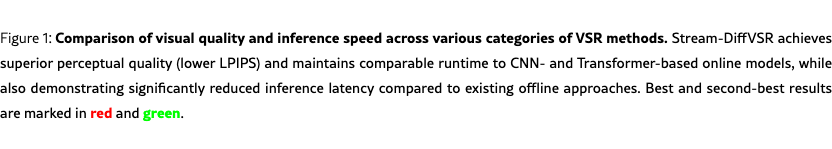
Fig. 1 illustrates the core advantage of our approach by comparing visual quality and runtime across various categories of video super-resolution methods. Our Stream-DiffVSR achieves superior perceptual quality (measured by LPIPS [96]) and temporal consistency, outperforming existing unidirectional CNN- and Transformer-based methods (e.g., MIA-VSR [105], RealViformer [98], TMP [99]). Notably, Stream-DiffVSR offers significantly faster per-frame inference than prior diffusion-based approaches (e.g., StableVSR [58], MGLD-VSR [89]), attributed to our use of a distilled 4-step denoising process and a lightweight temporal-aware decoder.

In addition, existing diffusion-based methods, such as StableVSR [58] typically rely on bidirectional or future-frame information, resulting in prohibitively high processing latency that is not suitable for online scenarios. Specifically, for a 100-frame video, StableVSR (46.2 s/frame) would incur an initial latency exceeding 4600 seconds on an RTX 4090 GPU, as it requires processing the entire sequence before generating even the first output frame. In contrast, our Stream-DiffVSR operates in a strictly causal, autoregressive manner, conditioning only on the immediately preceding frame. Consequently, the initial frame latency of Stream-DiffVSR corresponds to a single frame’s inference time (0.328 s/frame), reducing the latency by more than three orders of magnitude compared to StableVSR. This significant latency reduction demonstrates that Stream-DiffVSR effectively unlocks the potential of diffusion models for practical, low-latency online video super-resolution.

S1.T1 — Table 1: Comparison of diffusion-based VSR methods. We report online capability, inference steps, runtime (FPS on 720p, RTX 4090), maximum end-to-end latency (sec), and whether each method uses distillation, temporal modeling, or offline future frames. OOM denotes out-of-memory, and - indicates missing public inference results. Notably, Stream-DiffVSR is the only diffusion-based method that runs in a strictly online, past-only setting with the lowest latency.

To summarize, the main contributions of this paper are:

•

We introduce the first diffusion-based framework explicitly designed for online, low-latency video super-resolution, achieving efficient inference through distillation from 50 denoising steps down to 4 steps.
•

We propose a novel Auto-regressive Temporal Guidance mechanism and a Temporal-aware Decoder to effectively leverage temporal information only from past frames, significantly enhancing perceptual quality and temporal consistency.
•

Extensive experiments demonstrate that our approach outperforms existing methods across key perceptual and temporal consistency metrics while achieving practical inference speeds, thereby making diffusion-based VSR applicable for real-world online scenarios.

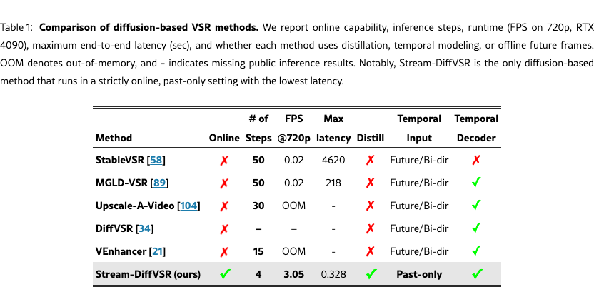
To contextualize our contributions, Table 1 compares recent diffusion-based VSR methods in terms of online inference capability, runtime efficiency, and temporal modeling. Our method uniquely achieves online low-latency inference while preserving high visual quality and temporal stability. This substantial latency reduction of over three orders of magnitude compared to prior diffusion-based VSR models demonstrates that Stream-DiffVSR is uniquely suited for low-latency online applications such as video conferencing and AR/VR.

2 Related Work

Video Super-resolution.

VSR methods reconstruct high-resolution videos from low-resolution inputs through CNN-based approaches [87, 70, 79, 4, 5, 68], deformable convolutions [70, 12, 107], online processing [99], recurrent architectures [61, 15, 25, 91, 33], flow-guided methods [92, 19, 43], and Transformer-based models [73, 37, 36, 63, 105]. Despite advances, low-latency online processing remains challenging.

Real-world Video Super-resolution.

Real-world VSR addresses unknown degradations [88, 6] through pre-cleaning modules [6, 18, 80, 44], online approaches [98], kernel estimation [54, 28], synthetic degradations [27, 65, 97, 7], new benchmarks [102, 11], real-time systems [3], advanced GANs [9, 72], and Transformer restorers [93, 35, 2]. Warp error-aware consistency [31] emphasizes temporal error regularisation.

Diffusion-based Image and Video Restoration.

Diffusion models provide powerful generative priors [55, 14, 8] for single-image SR [60, 32, 24], inpainting [47, 81, 40, 71], and quality enhancement [23, 16, 77]. Video diffusion methods include StableVSR [58], MGLD-VSR [89], DC-VSR [20], DOVE [10], UltraVSR [42], Upscale-A-Video [104], DiffVSR [34], DiffIR2VR-Zero [90], VideoGigaGAN [86], VEnhancer [21], temporal coherence [76], AVID [100], and SeedVR2 [78]. Auto-regressive approaches [67, 84, 39, 101] show promise. Acceleration techniques include consistency models [48, 17], advanced solvers [46, 45, 103], flow-based methods [41, 29], distillation [62, 50, 106, 85, 108], and efficient architectures [1]. Theoretical advances [74, 75] and recent image/offline distillation methods [66, 94, 82, 83] exist, but our Stream-DiffVSR uniquely applies distillation in strict online settings with causal temporal modeling for real-time VSR.

3 Method

We propose Stream-DiffVSR, a streamable auto-regressive diffusion framework for efficient video super-resolution (VSR). Its core innovation lies in an auto-regressive formulation that improves both temporal consistency and inference speed. The framework comprises: (1) a distilled few-step U-Net for accelerated diffusion inference, (2) Auto-regressive Temporal Guidance that conditions latent denoising on previously warped high-quality frames, and (3) an Auto-regressive Temporal-aware Decoder that explicitly incorporates temporal cues. Together, these components enable Stream-DiffVSR to produce stable and perceptually coherent videos.

3.1 Diffusion Models Preliminaries

Diffusion Models [22] transform complex data distributions into simpler Gaussian distributions via a forward diffusion process and reconstruct the original data using a learned reverse denoising process. The forward process gradually adds Gaussian noise to the initial data $x_{0}$ , forming a Markov chain: $q(x_{t}\mid x_{t-1})=\mathcal{N}\!\bigl(x_{t};\sqrt{1-\beta_{t}}\,x_{t-1},\,\beta_{t}I\bigr)$ for $t=1,\dots,T$ , where $\beta_{t}$ denotes a predefined noise schedule. At timestep $t$ , the noised data $x_{t}$ can be directly sampled from the clean data $x_{0}$ as: $x_{t}=\sqrt{\alpha_{t}}\,x_{0}+\sqrt{1-\alpha_{t}}\,\epsilon$ , where $\epsilon\sim\mathcal{N}(0,I)$ and $\alpha_{t}=\prod_{i=1}^{t}(1-\beta_{i})$ , where $\alpha_{t}=\prod_{i=1}^{t}(1-\beta_{i})$ . The reverse process progressively removes noise from $x_{T}$ , reconstructing the original data $x_{0}$ through a learned denoising operation modeled as a Markov chain, i.e., $p_{\theta}(x_{0},\dots,x_{T-1}\mid x_{T})=\prod_{t=1}^{T}p_{\theta}(x_{t-1}\mid x_{t})$ . Each individual step is parameterized by a neural network-based denoising function $p_{\theta}(x_{t-1}\mid x_{t})=\mathcal{N}\!\bigl(x_{t-1};\mu_{\theta}(x_{t},t),\Sigma_{\theta}(t)I\bigr)$ . Typically, the network predicts the noise component $\epsilon_{\theta}(x_{t},t)$ , from which the denoising mean is estimated as $\mu_{\theta}(x_{t},t)=\tfrac{1}{\sqrt{\alpha_{t}}}\Bigl(x_{t}-\tfrac{1-\alpha_{t}}{\sqrt{1-\alpha_{t}}}\,\epsilon_{\theta}(x_{t},t)\Bigr)$ . Latent Diffusion Models (LDMs) [57] further reduce computational complexity by projecting data into a lower-dimensional latent space using Variational Autoencoders (VAEs), significantly accelerating inference without sacrificing generative quality.

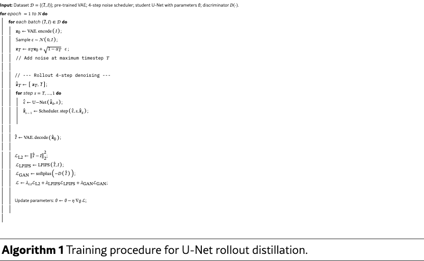
3.2 U-Net Rollout Distillation

We distill a pre-trained Stable Diffusion (SD) $\times$ 4 Upscaler [57, 56], originally designed for 50-step inference, into a 4-step variant that balances speed and perceptual quality. To mitigate the training–inference gap of timestep-sampling distillation, we adopt rollout distillation, where the U-Net performs the full 4-step denoising each iteration to obtain a clean latent. Detailed algorithms and implementation are provided in the supplementary material due to page limits.

Unlike conventional distillation that supervises random intermediate timesteps, our method applies loss only on the final denoised latent, ensuring the training trajectory mirrors inference and improving stability and alignment.

Our distillation requires no architectural changes. We train the U-Net by optimizing latent reconstruction with a loss that balances spatial accuracy, perceptual fidelity, and realism:

$\displaystyle\mathcal{L}_{\text{distill}}=$	$\displaystyle\,\\|\mathbf{z}_{\text{den}}-\mathbf{z}_{\text{gt}}\\|_{2}^{2}$	(1)
	$\displaystyle+\lambda_{\text{LPIPS}}\cdot\text{LPIPS}\left(D(\mathbf{z}_{\text{den}}),\mathbf{x}_{\text{gt}}\right)$
	$\displaystyle+\lambda_{\text{GAN}}\cdot\mathcal{L}_{\text{GAN}}\left(D(\mathbf{z}_{\text{den}})\right),$

where $\mathbf{z}_{\text{den}}$ and $\mathbf{z}_{\text{gt}}$ are the denoised and ground-truth latent representations. The decoder $D(\cdot)$ maps latent features back to RGB space for perceptual (LPIPS) and adversarial (GAN) loss calculations, encouraging visually realistic outputs.

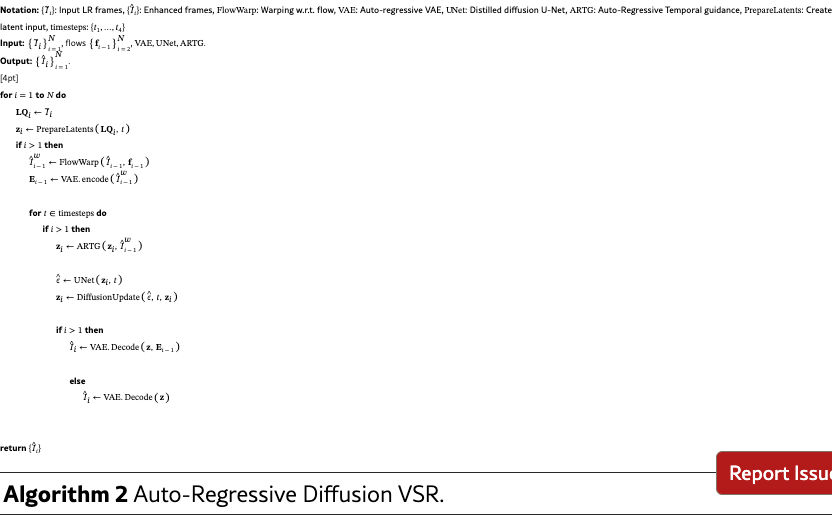
S3.F2 — Figure 2: Overview of Auto-regressive Temporal-aware Decoder. Given the denoised latent and warped previous frame, our decoder enhances temporal consistency using temporal processor modules. This module aligns and fuses these features via interpolation, convolution, and weighted fusion, effectively stabilizing detail reconstruction when decoding into the final RGB frame.

3.3 Auto-regressive Temporal Guidance

Leveraging temporal information is essential for capturing dynamics and ensuring frame continuity in video super-resolution. However, extensive temporal reasoning often incurs significant computational overhead, increasing per-frame inference time and system latency. Thus, efficient online VSR requires carefully balancing temporal utilization and computational cost to support low-latency processing.

To this end, we propose Auto-regressive Temporal Guidance (ARTG), which enforces temporal coherence during latent denoising. At each timestep $t$ , the U-Net takes both the current noised latent $z_{t}$ and the warped RGB frame from the previous output, $\hat{x}_{t-1}^{\text{warp}}=\text{Warp}(x_{t-1}^{\text{SR}},f_{t\leftarrow t-1})$ , where $f_{t\leftarrow t-1}$ is the optical flow from frame $t{-}1$ to $t$ . The denoising prediction is then formulated as:

\small\hat{\epsilon}_{\theta}=\text{UNet}(z_{t},t,\hat{x}_{t-1}^{\text{warp}}),

(2)

where the warped image $\hat{x}_{t-1}^{\text{warp}}$ serves as temporal conditioning input to guide the denoising process.

We train the ARTG module independently using consecutive pairs of low-quality and high-quality frames. The denoising U-Net and decoder are kept fixed during this stage, and the training objective focuses on reconstructing the target latent representation while preserving perceptual quality and visual realism. The total loss function is defined as:

$\displaystyle\mathcal{L}_{\text{ARTG}}=$	$\displaystyle\,\\|\mathbf{z}_{\text{den}}-\mathbf{z}_{\text{gt}}\\|_{2}^{2}$	(3)
	$\displaystyle+\lambda_{\text{LPIPS}}\cdot\text{LPIPS}(D(\mathbf{z}_{\text{den}}),\mathbf{x}_{\text{gt}})$
	$\displaystyle+\lambda_{\text{GAN}}\cdot\mathcal{L}_{\text{GAN}}(D(\mathbf{z}_{\text{den}})),$

where $\mathbf{z}_{\text{den}}$ denotes the denoised latent from DDIM updates with predicted noise $\hat{\boldsymbol{\epsilon}}_{\theta}$ , and $\mathbf{z}_{\text{gt}}$ is the ground-truth latent. The decoder $D(\cdot)$ maps latents to RGB, producing $D(\mathbf{z}_{\text{den}})$ for comparison with the ground-truth image $\mathbf{x}_{\text{gt}}$ . The latent $\ell_{2}$ loss enforces alignment, the perceptual loss preserves visual fidelity, and the adversarial loss promotes realism. This design leverages only past frames to propagate temporal context, improving consistency without additional latency.

S3.F3 — Figure 3:Training pipeline of Stream-DiffVSR. The training process consists of three sequential stages: (1) Distilling the denoising U-Net to reduce diffusion steps while maintaining perceptual quality with training objective (1); (2) Training the Temporal Processor Module (TPM) within the decoder to enhance temporal consistency at the RGB level with training objective (3); (3) Training the Auto-Regressive Temporal Guidance (ARTG) module to leverage previously restored high-quality frames for improved temporal coherence with training objective (6). Each module is trained separately before integrating them into the final framework.

S3.F4 — Figure 4:Overview of our pipeline. Given a low-quality (LQ) input frame, we first initialize its latent representation and employ an autoregressive diffusion model composed of a distilled denoising U-Net, autoregressive temporal Guidance, and an autoregressive temporal Decoder. Temporal guidance utilizes flow-warped high-quality (HQ) results from the previous frame to condition the current frame’s latent denoising and decoding processes, significantly improving perceptual quality and temporal consistency in an efficient, online manner.

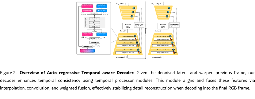
3.4 Auto-regressive Temporal-aware Decoder

Although the Auto-regressive Temporal Guidance (ARTG) improves temporal consistency in the latent space, the features produced by the Stable Diffusion $\times$ 4 Upscaler remain at one-quarter of the target resolution. This mismatch may introduce decoding artifacts or misalignment in dynamic scenes.

To address this issue, we propose an Auto-regressive Temporal-aware Decoder that incorporates temporal context into decoding to enhance spatial fidelity and temporal consistency. At timestep $t$ , the decoder takes the denoised latent $\mathbf{z}_{t}^{\text{den}}$ and the aligned feature $\hat{\mathbf{f}}_{t-1}$ derived from the previous super-resolved frame. Specifically, we compute:

\small\hat{\mathbf{x}}_{t-1}^{\text{warp}}=\text{Warp}(\mathbf{x}_{t-1}^{\text{SR}},f_{t\leftarrow t-1}),\,\,\,\,\hat{\mathbf{f}}_{t-1}=\text{Enc}(\hat{\mathbf{x}}_{t-1}^{\text{warp}}),

(4)

where $\mathbf{x}_{t-1}^{\text{SR}}$ is the previously generated RGB output, $f_{t\leftarrow t-1}$ is the optical flow from frame $t-1$ to $t$ , and $\text{Enc}(\cdot)$ is a frozen encoder that projects the warped image into the latent feature space.

The decoder then synthesizes the current frame using:

\small\mathbf{x}_{t}^{\text{SR}}=\text{Decoder}(\mathbf{z}_{t}^{\text{den}},\hat{\mathbf{f}}_{t-1}).

(5)

We adopt a multi-scale fusion strategy inside the decoder to combine current spatial information and prior temporal features across multiple resolution levels, as illustrated in Fig. 2. This design helps reinforce temporal coherence while recovering fine spatial details.

Temporal Processor Module (TPM).

We integrate TPM after each spatial convolutional layer in the decoder to explicitly inject temporal coherence, enhancing stability and continuity of reconstructed frames. These modules utilize latent features from the current frame and warped features from the previous frame, optimizing temporal consistency independently from spatial reconstruction. Our training objective for the TPM is defined as:

$\displaystyle\mathcal{L}_{\text{TPM}}=$	$\displaystyle\;\mathcal{L}_{\text{rec}}(\mathbf{x}_{t}^{\text{rec}},\mathbf{x}_{t}^{\text{GT}})$	(6)
	$\displaystyle+\lambda_{\text{flow}}\left\\|\text{OF}(\mathbf{x}_{t}^{\text{rec}},\mathbf{x}_{t-1}^{\text{rec}})-\text{OF}(\mathbf{x}_{t}^{\text{GT}},\mathbf{x}_{t-1}^{\text{GT}})\right\\|_{2}^{2}$
	$\displaystyle+\lambda_{\text{GAN}}\mathcal{L}_{\text{GAN}}(\mathbf{x}_{t}^{\text{rec}})$
	$\displaystyle+\lambda_{\text{LPIPS}}\text{LPIPS}(\mathbf{x}_{t}^{\text{rec}},\mathbf{x}_{t}^{\text{GT}}),$

where $\mathbf{x}_{t}^{\text{SR}}\in\mathbb{R}^{3\times H\times W}$ is the predicted frame at time $t$ , and $\mathbf{x}_{t}^{\text{GT}}$ is the ground-truth frame. The reconstruction loss $\mathcal{L}_{\text{rec}}=\text{SmoothL1}(\mathbf{x}_{t}^{\text{rec}},\mathbf{x}_{t}^{\text{GT}})$ enforces spatial fidelity, the adversarial loss $\mathcal{L}_{\text{GAN}}$ improves realism, and the optical-flow term $\text{OF}(\cdot,\cdot)$ reduces temporal discrepancies, yielding consistent and perceptually faithful outputs.

S3.T2 — Table 2: Quantitative comparison against bidirectional/offline methods on the REDS4 dataset. We compare CNN-, Transformer-, and diffusion-based methods on REDS4. Stream-DiffVSR achieves superior perceptual and temporal quality with high stability across sequences. ↑ indicates higher is better; ↓ indicates lower is better. Dir. denotes temporal direction: B for bidirectional/offline, U for unidirectional/online. Runtime is measured per 720p frame on an RTX 4090. Latency-max denotes the maximum end-to-end latency measured over 100-frame video sequences, providing a fair comparison with offline methods whose initial delay scales with sequence length. tLP and tOF are scaled by 100× and 10×. Best and second-best results are marked in red and blue.

S3.T3 — Table 3: Quantitative comparison against unidirectional/online methods on the REDS4 dataset.

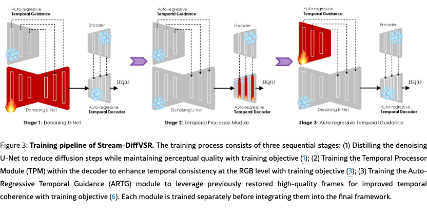
3.5 Training and Inference Stages

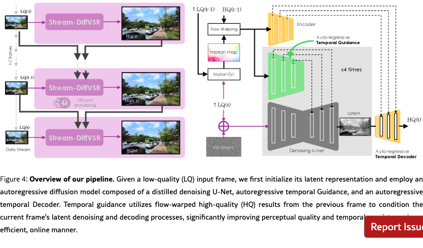
Our training pipeline consists of three independent stages (Fig. 3), while our inference process and the Auto-Regressive Diffusion-based VSR algorithm are illustrated in Fig. 4 and detailed in the appendix due to page constraints, respectively.

Distilling the Denoising U-Net.

We first distill the denoising U-Net using pairs of low-quality (LQ) and high-quality (HQ) frames to optimize per-frame super-resolution and latent-space consistency.

Training the Temporal Processor Module (TPM).

In parallel, we train the Temporal Processor Module (TPM) in the decoder using ground-truth frames, keeping all other weights fixed. This enhances the decoder’s capability to incorporate temporal information into the final RGB reconstruction.

Training Auto-regressive Temporal Guidance.

After training and freezing the U-Net and decoder, we train the ARTG, which leverages flow-aligned previous outputs to enhance temporal coherence without degrading spatial quality. This staged training strategy progressively refines spatial fidelity, latent consistency, and temporal smoothness in a decoupled manner.

Inference.

Given a sequence of low-quality (LQ) frames, our method auto-regressively generates high-quality (HQ) outputs. For each frame $t$ , denoising is conditioned on the previous output $HQ_{t-1}$ , warped via optical flow to capture temporal motion. To balance quality and efficiency, we employ a 4-step DDIM scheme using a distilled U-Net. By combining motion alignment with reduced denoising steps, our inference pipeline achieves efficient and stable temporal consistency.

4 Experiment

Due to space limitations, we provide the experimental setup in the appendix.

S4.T4 — Table 4: Quantitative comparison against bidirectional/offline methods on the Vimeo-90K-T dataset. Stream-DiffVSR surpasses other bidirectional methods in perceptual quality, temporal consistency, and runtime. Runtime is the average per-frame inference time (seconds) on 448×256 videos using an RTX 4090. Best and second-best results are shown in red and blue.

S4.T5 — Table 5: Quantitative comparison against unidirectional/online methods on the Vimeo-90K-T dataset.

S4.T6 — Table 6:Memory and inference speed comparison on NVIDIA A6000. OOM = out of memory. Our method achieves the lowest memory footprint, fastest runtime, and lowest latency.

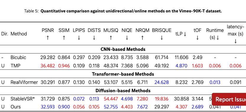
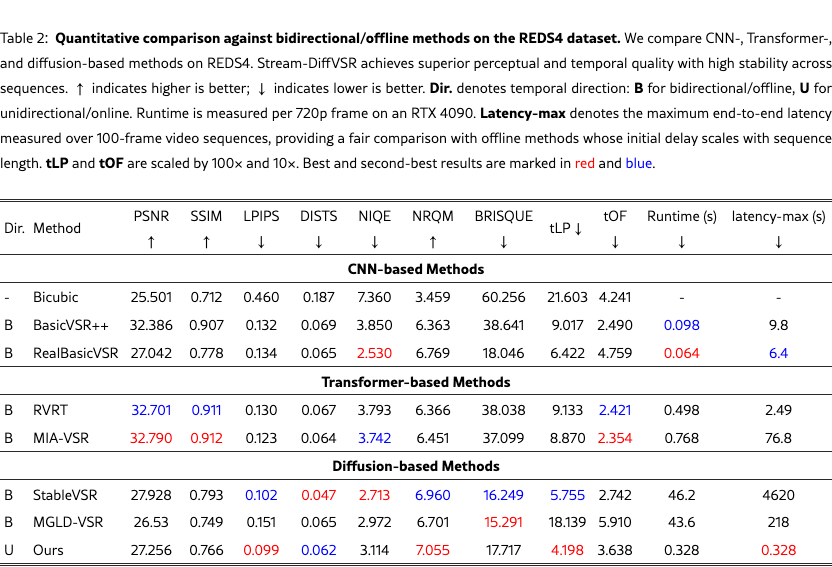
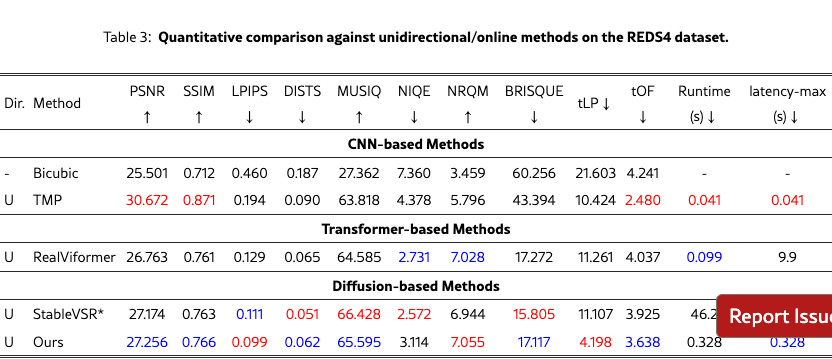
We quantitatively compare Stream-DiffVSR with state-of-the-art VSR methods on REDS4, Vimeo-90K-T, VideoLQ, and Vid4, covering diverse scene content and motion characteristics. Tabs. 2 and 4 report results across CNN-, Transformer-, and diffusion-based approaches under both bidirectional (offline) and unidirectional (online) settings.

On REDS4, Stream-DiffVSR achieves superior perceptual quality (LPIPS=0.099) over CNN (BasicVSR++, RealBasicVSR), Transformer (RVRT), and diffusion-based methods (StableVSR, MGLD-VSR), while also delivering competitive temporal consistency (tLP=4.198, tOF=3.638). Notably, it attains these gains with substantially lower runtime (0.328s/frame vs. 43–46s/frame for diffusion models).

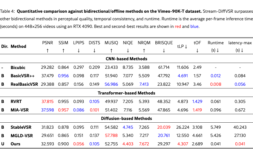
On Vimeo-90K-T, Stream-DiffVSR likewise attains leading perceptual performance (LPIPS=0.056, DISTS=0.105) and improved temporal consistency (tLP=4.307, tOF=2.689) with a competitive runtime of 0.041s/frame, highlighting its suitability for online deployment.

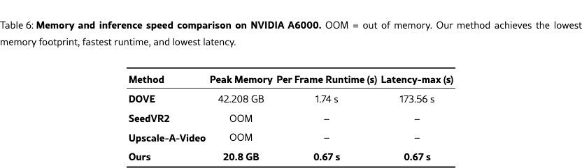
In addition to speed, Stream-DiffVSR achieves a markedly lower memory footprint. As shown in Tab. 6, prior diffusion-based VSR methods such as DOVE, SeedVR2, and Upscale-A-Video either require over 42 GB of GPU memory or fail with out-of-memory errors on an NVIDIA A6000. In contrast, Stream-DiffVSR operates within 20.8 GB while running more than $2.5\times$ faster, underscoring its efficiency and deployability.

Results on VideoLQ and Vid4 further confirm strong perceptual and temporal performance, demonstrating robust generalization across the entire evaluation dataset.

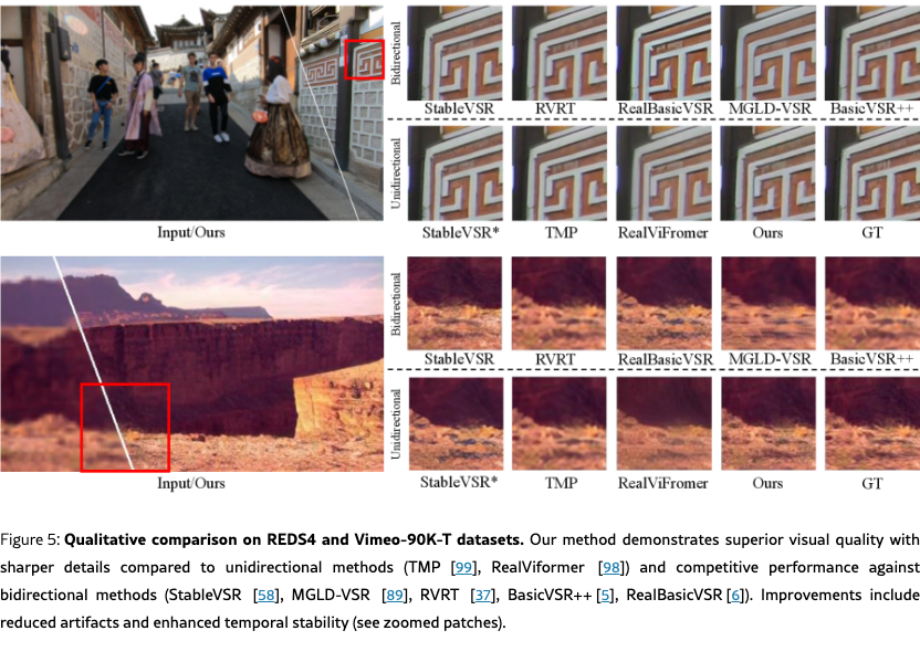
S4.F5 — Figure 5:Qualitative comparison on REDS4 and Vimeo-90K-T datasets. Our method demonstrates superior visual quality with sharper details compared to unidirectional methods (TMP [99], RealViformer [98]) and competitive performance against bidirectional methods (StableVSR [58], MGLD-VSR [89], RVRT [37], BasicVSR++[5], RealBasicVSR[6]). Improvements include reduced artifacts and enhanced temporal stability (see zoomed patches).

4.1 Qualitative Comparisons

We provide qualitative comparisons in Fig. 5, where Stream-DiffVSR generates sharper details and fewer artifacts than prior methods. Additional visualizations of temporal consistency and flow coherence are included in the supplemental material. A qualitative comparison with Upscale-A-Video (UAV) [104] is included in the appendix.

S4.T7 — Table 7:Ablation study of temporal modules in Stream-DiffVSR.

S4.T8 — Table 8:Ablation study on training strategy.

S4.T9 — Table 9:Ablation study on denoising step count within Stream-DiffVSR. We evaluate 50, 10, 1, and 4 steps. Our 4-step design achieves a favorable balance between perceptual quality and runtime.

S4.T10 — Table 10:Ablation study on Rollout Training. Comparison of random timestep distillation vs. rollout training across fidelity and perceptual metrics.

S4.F8 — Figure 6:Ablation study on the Temporal Processor Module (TPM). Integrating TPM improves motion stability and reduces temporal artifacts by leveraging warped previous-frame features, enhancing temporal consistency in video super-resolution.

S4.F8.3 — Figure 7:Ablation study on inference steps. The 4-step model yields the best quality–efficiency trade-off, validating our distillation strategy.

S4.F8.3.2 — Figure 8:Ablation study on Auto-regressive Temporal Guidance (ARTG). ARTG enhances temporal consistency and perceptual quality by leveraging warped previous frames, reducing flickering, and improving structural coherence.

4.2 Ablation Study

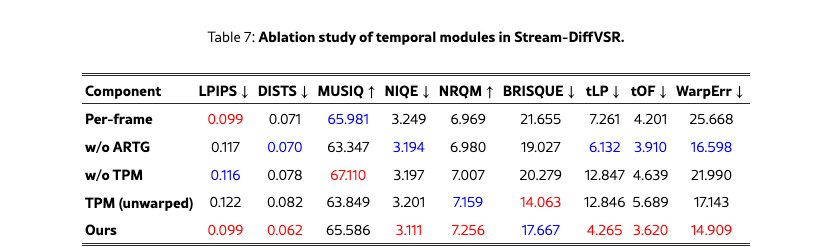
We ablate key components of Stream-DiffVSR including denoising-step reduction, ARTG, TPM, timestep selection, and training-stage combinations on REDS4 to ensure consistent evaluation of perceptual quality and temporal stability.

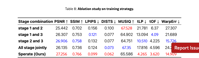
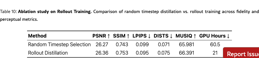
We perform ablation studies on training strategies in Tab. 10 and Tab. 8. For stage-wise training, partial or joint training yields inferior results, while our separate stage-wise scheme achieves the best trade-off across fidelity, perceptual, and temporal metrics. For distillation, rollout training outperforms random timestep selection in both quality and efficiency, reducing training cost from 60.5 to 21 GPU hours on 4×A6000 GPUs.

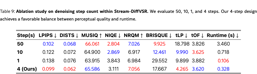
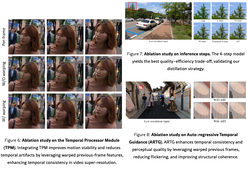
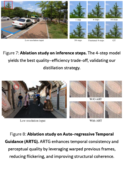
We assess the runtime–quality trade-off by varying DDIM inference steps while keeping model weights fixed. As shown in Tab. 9 and Fig. 8, fewer steps increase efficiency but reduce perceptual quality, whereas more steps improve fidelity with higher latency. A 4-step setting provides the best balance.

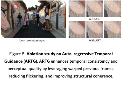
Tab. 7 and Fig. 8 show the effectiveness of ARTG and TPM. The per-frame baseline uses only the distilled U-Net with both ARTG and TPM disabled. In the ablation labels, w/o indicates that a module is fully removed; for instance, TPM (unwarp) feeds TPM the previous HR frame without flow-based warping, removing motion alignment. ARTG improves perceptual quality (LPIPS 0.117→0.099) and temporal consistency (tLP100 6.132→4.265). TPM further enhances temporal coherence through temporal-feature warping and fusion, yielding additional gains in tLP100. These results highlight the complementary roles of latent-space guidance and decoder-side temporal modeling.

5 Conclusion

We propose Stream-DiffVSR, an efficient online video super-resolution framework using diffusion models. By integrating a distilled U-Net, Auto-Regressive Temporal Guidance, and Temporal-aware Decoder, Stream-DiffVSR achieves superior perceptual quality, temporal consistency, and practical inference speed for low-latency applications.

Limitations.

Stream-DiffVSR remains heavier than CNN and Transformer models, and its use of optical flow can introduce fast-motion artifacts. Its auto-regressive design also weakens initial frames, indicating a need for better initialization. Improving robustness to real-world degradations remains important.

Acknowledgements.

This research was funded by the National Science and Technology Council, Taiwan, under Grants NSTC 112-2222-E-A49-004-MY2 and 113-2628-E-A49-023-. The authors are grateful to Google, NVIDIA, and MediaTek Inc. for their generous donations. Yu-Lun Liu acknowledges the Yushan Young Fellow Program by the MOE in Taiwan.

References

Bai et al. [2025] Weimin Bai, Suzhe Xu, Yiwei Ren, Jinhua Hao, Ming Sun, Wenzheng Chen, and He Sun. Instantvir: Real-time video inverse problem solver with distilled diffusion prior. arXiv preprint arXiv:2511.14208, 2025.
Blau and Michaeli [2018] Yochai Blau and Tomer Michaeli. The perception-distortion tradeoff. In Proceedings of the IEEE Conference on Computer Vision and Pattern Recognition, pages 6228–6237, 2018.
Cao et al. [2021] Yanpeng Cao, Chengcheng Wang, Changjun Song, Yongming Tang, and He Li. Real-time super-resolution system of 4k-video based on deep learning. In 2021 IEEE 32nd International Conference on Application-specific Systems, Architectures and Processors (ASAP), pages 69–76. IEEE, 2021.
Chan et al. [2021] Kelvin CK Chan, Xintao Wang, Ke Yu, Chao Dong, and Chen Change Loy. Basicvsr: The search for essential components in video super-resolution and beyond. In Proceedings of the IEEE/CVF Conference on Computer Vision and Pattern Recognition, pages 4947–4956, 2021.
Chan et al. [2022a] Kelvin CK Chan, Shangchen Zhou, Xiangyu Xu, and Chen Change Loy. Basicvsr++: Improving video super-resolution with enhanced propagation and alignment. In Proceedings of the IEEE/CVF conference on computer vision and pattern recognition, pages 5972–5981, 2022a.
Chan et al. [2022b] Kelvin CK Chan, Shangchen Zhou, Xiangyu Xu, and Chen Change Loy. Investigating tradeoffs in real-world video super-resolution. In Proceedings of the IEEE/CVF Conference on Computer Vision and Pattern Recognition, pages 5962–5971, 2022b.
Chang et al. [2020] Ke-Chi Chang, Ren Wang, Hung-Jin Lin, Yu-Lun Liu, Chia-Ping Chen, Yu-Lin Chang, and Hwann-Tzong Chen. Learning camera-aware noise models. In European Conference on Computer Vision, pages 343–358. Springer, 2020.
Chao et al. [2022] Chen-Hao Chao, Wei-Fang Sun, Bo-Wun Cheng, Yi-Chen Lo, Chia-Che Chang, Yu-Lun Liu, Yu-Lin Chang, Chia-Ping Chen, and Chun-Yi Lee. Denoising likelihood score matching for conditional score-based data generation. arXiv preprint arXiv:2203.14206, 2022.
Chen et al. [2024] Rui Chen, Yang Mu, and Yan Zhang. High-order relational generative adversarial network for video super-resolution. Pattern Recognition, 146:110059, 2024.
Chen et al. [2025] Zheng Chen, Zichen Zou, Kewei Zhang, Xiongfei Su, Xin Yuan, Yong Guo, and Yulun Zhang. Dove: Efficient one-step diffusion model for real-world video super-resolution. arXiv preprint arXiv:2505.16239, 2025.
Conde et al. [2024] Marcos V Conde, Zhijun Lei, Wen Li, Christos Bampis, Ioannis Katsavounidis, Radu Timofte, Qing Luo, Jie Song, Linyan Jiang, Haibo Lei, et al. Aim 2024 challenge on efficient video super-resolution for av1 compressed content. In European Conference on Computer Vision, pages 304–325. Springer, 2024.
Dai et al. [2017] Jifeng Dai, Haozhi Qi, Yuwen Xiong, Yi Li, Guodong Zhang, Han Hu, and Yichen Wei. Deformable convolutional networks. In Proceedings of the IEEE international conference on computer vision (ICCV), pages 764–773, 2017.
Ding et al. [2020] Keyan Ding, Kede Ma, Shiqi Wang, and Eero P Simoncelli. Image quality assessment: Unifying structure and texture similarity. IEEE transactions on pattern analysis and machine intelligence, 44(5):2567–2581, 2020.
Esser et al. [2021] Patrick Esser, Robin Rombach, and Bjorn Ommer. Taming transformers for high-resolution image synthesis. In Proceedings of the IEEE/CVF conference on computer vision and pattern recognition, pages 12873–12883, 2021.
Fuoli et al. [2019] Dario Fuoli, Shuhang Gu, and Radu Timofte. Efficient video super-resolution through recurrent latent space propagation. In 2019 IEEE/CVF International Conference on Computer Vision Workshop (ICCVW), pages 3476–3485. IEEE, 2019.
Gao et al. [2023] Sicheng Gao, Xuhui Liu, Bohan Zeng, Sheng Xu, Yanjing Li, Xiaoyan Luo, Jianzhuang Liu, Xiantong Zhen, and Baochang Zhang. Implicit diffusion models for continuous super-resolution. In Proceedings of the IEEE/CVF conference on computer vision and pattern recognition, pages 10021–10030, 2023.
Geng et al. [2024] Zhengyang Geng, Ashwini Pokle, William Luo, Justin Lin, and J Zico Kolter. Consistency models made easy. arXiv preprint arXiv:2406.14548, 2024.
Goodfellow et al. [2020] Ian Goodfellow, Jean Pouget-Abadie, Mehdi Mirza, Bing Xu, David Warde-Farley, Sherjil Ozair, Aaron Courville, and Yoshua Bengio. Generative adversarial networks. Communications of the ACM, 63(11):139–144, 2020.
Guo et al. [2024] Zujin Guo, Wei Li, and Chen Change Loy. Generalizable implicit motion modeling for video frame interpolation. Advances in Neural Information Processing Systems, 37:63747–63770, 2024.
Han et al. [2025] Janghyeok Han, Gyujin Sim, Geonung Kim, Hyun-Seung Lee, Kyuha Choi, Youngseok Han, and Sunghyun Cho. Dc-vsr: Spatially and temporally consistent video super-resolution with video diffusion prior. In Proceedings of the Special Interest Group on Computer Graphics and Interactive Techniques Conference Conference Papers, pages 1–11, 2025.
He et al. [2024] Jingwen He, Tianfan Xue, Dongyang Liu, Xinqi Lin, Peng Gao, Dahua Lin, Yu Qiao, Wanli Ouyang, and Ziwei Liu. Venhancer: Generative space-time enhancement for video generation. arXiv preprint arXiv:2407.07667, 2024.
Ho et al. [2020] Jonathan Ho, Ajay Jain, and Pieter Abbeel. Denoising diffusion probabilistic models. Advances in neural information processing systems, 33:6840–6851, 2020.
Ho et al. [2022] Jonathan Ho, Chitwan Saharia, William Chan, David J Fleet, Mohammad Norouzi, and Tim Salimans. Cascaded diffusion models for high fidelity image generation. Journal of Machine Learning Research, 23(47):1–33, 2022.
Hsiao et al. [2024] Chi-Wei Hsiao, Yu-Lun Liu, Cheng-Kun Yang, Sheng-Po Kuo, Kevin Jou, and Chia-Ping Chen. Ref-ldm: A latent diffusion model for reference-based face image restoration. Advances in Neural Information Processing Systems, 37:74840–74867, 2024.
Isobe et al. [2020] Takashi Isobe, Xu Jia, Shuhang Gu, Songjiang Li, Shengjin Wang, and Qi Tian. Video super-resolution with recurrent structure-detail network. arXiv preprint arXiv:2008.00455, 2020.
Isola et al. [2017] Phillip Isola, Jun-Yan Zhu, Tinghui Zhou, and Alexei A Efros. Image-to-image translation with conditional adversarial networks. In Proceedings of the IEEE conference on computer vision and pattern recognition, pages 1125–1134, 2017.
Jeelani et al. [2023] Mehran Jeelani, Noshaba Cheema, Klaus Illgner-Fehns, Philipp Slusallek, Sunil Jaiswal, et al. Expanding synthetic real-world degradations for blind video super resolution. In Proceedings of the IEEE/CVF conference on computer vision and pattern recognition, pages 1199–1208, 2023.
Ji et al. [2020] Xiaozhong Ji, Yun Cao, Ying Tai, Chengjie Wang, Jilin Li, and Feiyue Huang. Real-world super-resolution via kernel estimation and noise injection. In proceedings of the IEEE/CVF conference on computer vision and pattern recognition workshops, pages 466–467, 2020.
Jin et al. [2024] Yang Jin, Zhicheng Sun, Ningyuan Li, Kun Xu, Hao Jiang, Nan Zhuang, Quzhe Huang, Yang Song, Yadong Mu, and Zhouchen Lin. Pyramidal flow matching for efficient video generative modeling. arXiv preprint arXiv:2410.05954, 2024.
Ke et al. [2021] Junjie Ke, Qifei Wang, Yilin Wang, Peyman Milanfar, and Feng Yang. Musiq: Multi-scale image quality transformer. In Proceedings of the IEEE/CVF International Conference on Computer Vision, pages 5148–5157, 2021.
Lei et al. [2020] Chenyang Lei, Yazhou Xing, and Qifeng Chen. Blind video temporal consistency via deep video prior. Advances in Neural Information Processing Systems, 33:1083–1093, 2020.
Li et al. [2022] Haoying Li, Yifan Yang, Meng Chang, Shiqi Chen, Huajun Feng, Zhihai Xu, Qi Li, and Yueting Chen. Srdiff: Single image super-resolution with diffusion probabilistic models. Neurocomputing, 479:47–59, 2022.
Li et al. [2020] Wenbo Li, Xin Tao, Taian Guo, Lu Qi, Jiangbo Lu, and Jiaya Jia. Mucan: Multi-correspondence aggregation network for video super-resolution. arXiv preprint arXiv:2007.11803, 2020.
Li et al. [2025] Xiaohui Li, Yihao Liu, Shuo Cao, Ziyan Chen, Shaobin Zhuang, Xiangyu Chen, Yinan He, Yi Wang, and Yu Qiao. Diffvsr: Enhancing real-world video super-resolution with diffusion models for advanced visual quality and temporal consistency. arXiv preprint arXiv:2501.10110, 2025.
Liang et al. [2021] Jingyun Liang, Jiezhang Cao, Guolei Sun, Kai Zhang, Luc Van Gool, and Radu Timofte. Swinir: Image restoration using swin transformer. In Proceedings of the IEEE/CVF international conference on computer vision, pages 1833–1844, 2021.
Liang et al. [2022a] Jingyun Liang, Jiezhang Cao, Yuchen Fan, Kai Zhang, Rakesh Ranjan, Yawei Li, Radu Timofte, and Luc Van Gool. Vrt: A video restoration transformer. arXiv preprint arXiv:2201.12288, 2022a.
Liang et al. [2022b] Jingyun Liang, Yuchen Fan, Xiaoyu Xiang, Rakesh Ranjan, Eddy Ilg, Simon Green, Jiezhang Cao, Kai Zhang, Radu Timofte, and Luc V Gool. Recurrent video restoration transformer with guided deformable attention. Advances in Neural Information Processing Systems, 35:378–393, 2022b.
Liu and Sun [2013] Ce Liu and Deqing Sun. On bayesian adaptive video super resolution. IEEE transactions on pattern analysis and machine intelligence, 36(2):346–360, 2013.
Liu et al. [2024] Haozhe Liu, Shikun Liu, Zijian Zhou, Mengmeng Xu, Yanping Xie, Xiao Han, Juan C Pérez, Ding Liu, Kumara Kahatapitiya, Menglin Jia, et al. Mardini: Masked autoregressive diffusion for video generation at scale. arXiv preprint arXiv:2410.20280, 2024.
Liu et al. [2025a] Kuan-Hung Liu, Cheng-Kun Yang, Min-Hung Chen, Yu-Lun Liu, and Yen-Yu Lin. Corrfill: Enhancing faithfulness in reference-based inpainting with correspondence guidance in diffusion models. In 2025 IEEE/CVF Winter Conference on Applications of Computer Vision (WACV), pages 1618–1627. IEEE, 2025a.
Liu et al. [2023] Xingchao Liu, Xiwen Zhang, Jianzhu Ma, Jian Peng, et al. Instaflow: One step is enough for high-quality diffusion-based text-to-image generation. In The Twelfth International Conference on Learning Representations, 2023.
Liu et al. [2025b] Yong Liu, Jinshan Pan, Yinchuan Li, Qingji Dong, Chao Zhu, Yu Guo, and Fei Wang. Ultravsr: Achieving ultra-realistic video super-resolution with efficient one-step diffusion space. arXiv preprint arXiv:2505.19958, 2025b.
Liu et al. [2019] Yu-Lun Liu, Yi-Tung Liao, Yen-Yu Lin, and Yung-Yu Chuang. Deep video frame interpolation using cyclic frame generation. In Proceedings of the AAAI Conference on Artificial Intelligence, pages 8794–8802, 2019.
Liu et al. [2021] Yu-Lun Liu, Wei-Sheng Lai, Ming-Hsuan Yang, Yung-Yu Chuang, and Jia-Bin Huang. Learning to see through obstructions with layered decomposition. IEEE transactions on pattern analysis and machine intelligence, 44(11):8387–8402, 2021.
Lu et al. [2025] Cheng Lu, Yuhao Zhou, Fan Bao, Jianfei Chen, Chongxuan Li, and Jun Zhu. Dpm-solver++: Fast solver for guided sampling of diffusion probabilistic models. Machine Intelligence Research, pages 1–22, 2025.
Lu et al. [2022] Cheng Lu et al. Dpm-solver: A fast ode solver for diffusion probabilistic model sampling in around 10 steps. NeurIPS, 35:5775–5787, 2022.
Lugmayr et al. [2022] Andreas Lugmayr, Martin Danelljan, Andres Romero, Fisher Yu, Radu Timofte, and Luc Van Gool. Repaint: Inpainting using denoising diffusion probabilistic models. In Proceedings of the IEEE/CVF Conference on Computer Vision and Pattern Recognition, pages 11461–11471, 2022.
Luo et al. [2023] Simian Luo et al. Latent consistency models: Synthesizing high-resolution images with few-step inference. arXiv preprint arXiv:2310.04378, 2023.
Ma et al. [2017] Chao Ma, Chih-Yuan Yang, Xiaokang Yang, and Ming-Hsuan Yang. Learning a no-reference quality metric for single-image super-resolution. Computer Vision and Image Understanding, 158:1–16, 2017.
Meng et al. [2023] Chenlin Meng, Robin Rombach, Ruiqi Gao, Diederik Kingma, Stefano Ermon, Jonathan Ho, and Tim Salimans. On distillation of guided diffusion models. In Proceedings of the IEEE/CVF Conference on Computer Vision and Pattern Recognition, pages 14297–14306, 2023.
Mittal et al. [2012] Anish Mittal, Anush Krishna Moorthy, and Alan Conrad Bovik. No-reference image quality assessment in the spatial domain. IEEE Transactions on image processing, 21(12):4695–4708, 2012.
Nah et al. [2019a] Seungjun Nah, Sungyong Baik, Seokil Hong, Gyeongsik Moon, Sanghyun Son, Radu Timofte, and Kyoung Mu Lee. Ntire 2019 challenge on video deblurring and super-resolution: Dataset and study. In CVPR Workshops, 2019a.
Nah et al. [2019b] Seungjun Nah, Sungyong Baik, Seokil Hong, Gyeongsik Moon, Sanghyun Son, Radu Timofte, and Kyoung Mu Lee. Ntire 2019 challenge on video deblurring and super-resolution: Dataset and study. In CVPRW, 2019b.
Pan et al. [2021] Jinshan Pan, Haoran Bai, Jiangxin Dong, Jiawei Zhang, and Jinhui Tang. Deep blind video super-resolution. In Proceedings of the IEEE/CVF International Conference on Computer Vision, pages 4811–4820, 2021.
Rombach et al. [2021] Robin Rombach, Andreas Blattmann, Dominik Lorenz, Patrick Esser, and Björn Ommer. High-resolution image synthesis with latent diffusion models, 2021.
Rombach et al. [2022a] Robin Rombach, Andreas Blattmann, Dominik Lorenz, Patrick Esser, and Björn Ommer. High-resolution image synthesis with latent diffusion models. In Proceedings of the IEEE/CVF Conference on Computer Vision and Pattern Recognition (CVPR), pages 10684–10695, 2022a.
Rombach et al. [2022b] Robin Rombach, Andreas Blattmann, Dominik Lorenz, Patrick Esser, and Björn Ommer. High-resolution image synthesis with latent diffusion models. In Proceedings of the IEEE/CVF conference on computer vision and pattern recognition, pages 10684–10695, 2022b.
Rota et al. [2024] Claudio Rota, Marco Buzzelli, and Joost van de Weijer. Enhancing perceptual quality in video super-resolution through temporally-consistent detail synthesis using diffusion models. In European Conference on Computer Vision, pages 36–53. Springer, 2024.
Saad and Bovik [2012] Michele A Saad and Alan C Bovik. Blind quality assessment of videos using a model of natural scene statistics and motion coherency. In 2012 Conference Record of the Forty Sixth Asilomar Conference on Signals, Systems and Computers (ASILOMAR), pages 332–336. IEEE, 2012.
Saharia et al. [2022] Chitwan Saharia, Jonathan Ho, William Chan, Tim Salimans, David J Fleet, and Mohammad Norouzi. Image super-resolution via iterative refinement. IEEE transactions on pattern analysis and machine intelligence, 45(4):4713–4726, 2022.
Sajjadi et al. [2018] Mehdi SM Sajjadi, Raviteja Vemulapalli, and Matthew Brown. Frame-recurrent video super-resolution. In Proceedings of the IEEE conference on computer vision and pattern recognition, pages 6626–6634, 2018.
Salimans and Ho [2022] Tim Salimans and Jonathan Ho. Progressive distillation for fast sampling of diffusion models. arXiv preprint arXiv:2202.00512, 2022.
Shi et al. [2022] Shuwei Shi, Jinjin Gu, Liangbin Xie, Xintao Wang, Yujiu Yang, and Chao Dong. Rethinking alignment in video super-resolution transformers. arXiv preprint arXiv:2207.08494, 2022.
Song et al. [2020] Jiaming Song, Chenlin Meng, and Stefano Ermon. Denoising diffusion implicit models. arXiv preprint arXiv:2010.02502, 2020.
Song et al. [2024] Yexing Song, Meilin Wang, Zhijing Yang, Xiaoyu Xian, and Yukai Shi. Negvsr: Augmenting negatives for generalized noise modeling in real-world video super-resolution. In Proceedings of the AAAI Conference on Artificial Intelligence, pages 10705–10713, 2024.
Sun et al. [2025a] Lingchen Sun, Rongyuan Wu, Zhiyuan Ma, Shuaizheng Liu, Qiaosi Yi, and Lei Zhang. Pixel-level and semantic-level adjustable super-resolution: A dual-lora approach. 2025a.
Sun et al. [2025b] Mingzhen Sun, Weining Wang, Gen Li, Jiawei Liu, Jiahui Sun, Wanquan Feng, Shanshan Lao, SiYu Zhou, Qian He, and Jing Liu. Ar-diffusion: Asynchronous video generation with auto-regressive diffusion. In Proceedings of the Computer Vision and Pattern Recognition Conference, pages 7364–7373, 2025b.
Sun et al. [2025c] Yang-Che Sun, Cheng Yu Yeo, Ernie Chu, Jun-Cheng Chen, and Yu-Lun Liu. Fiper: Factorized features for robust image super-resolution and compression. In The Thirty-ninth Annual Conference on Neural Information Processing Systems, 2025c.
Teed and Deng [2020] Zachary Teed and Jia Deng. Raft: Recurrent all-pairs field transforms for optical flow. In Computer Vision–ECCV 2020: 16th European Conference, Glasgow, UK, August 23–28, 2020, Proceedings, Part II 16, pages 402–419. Springer, 2020.
Tian et al. [2020] Yapeng Tian, Yulun Zhang, Yun Fu, and Chenliang Xu. Tdan: Temporally-deformable alignment network for video super-resolution. In Proceedings of the IEEE/CVF Conference on Computer Vision and Pattern Recognition (CVPR), pages 3360–3369, 2020.
Tsai et al. [2025] Shr-Ruei Tsai, Wei-Cheng Chang, Jie-Ying Lee, Chih-Hai Su, and Yu-Lun Liu. Lightsout: Diffusion-based outpainting for enhanced lens flare removal. In Proceedings of the IEEE/CVF International Conference on Computer Vision, pages 6353–6363, 2025.
Tsai et al. [2023] Yu-Ju Tsai, Yu-Lun Liu, Lu Qi, Kelvin CK Chan, and Ming-Hsuan Yang. Dual associated encoder for face restoration. arXiv preprint arXiv:2308.07314, 2023.
Vaswani et al. [2017] Ashish Vaswani, Noam Shazeer, Niki Parmar, Jakob Uszkoreit, Llion Jones, Aidan N Gomez, Łukasz Kaiser, and Illia Polosukhin. Attention is all you need. Advances in neural information processing systems, 30, 2017.
Wang et al. [2024a] Fu-Yun Wang, Zhaoyang Huang, Alexander Bergman, Dazhong Shen, Peng Gao, Michael Lingelbach, Keqiang Sun, Weikang Bian, Guanglu Song, Yu Liu, et al. Phased consistency models. Advances in neural information processing systems, 37:83951–84009, 2024a.
Wang et al. [2024b] Fu-Yun Wang, Ling Yang, Zhaoyang Huang, Mengdi Wang, and Hongsheng Li. Rectified diffusion: Straightness is not your need in rectified flow. arXiv preprint arXiv:2410.07303, 2024b.
Wang et al. [2025a] Hengkang Wang, Yang Liu, Huidong Liu, Chien-Chih Wang, Yanhui Guo, Hongdong Li, Bryan Wang, and Ju Sun. Temporal-consistent video restoration with pre-trained diffusion models. arXiv preprint arXiv:2503.14863, 2025a.
Wang et al. [2024c] Jianyi Wang, Zongsheng Yue, Shangchen Zhou, Kelvin CK Chan, and Chen Change Loy. Exploiting diffusion prior for real-world image super-resolution. International Journal of Computer Vision, 132(12):5929–5949, 2024c.
Wang et al. [2025b] Jianyi Wang, Shanchuan Lin, Zhijie Lin, Yuxi Ren, Meng Wei, Zongsheng Yue, Shangchen Zhou, Hao Chen, Yang Zhao, Ceyuan Yang, et al. Seedvr2: One-step video restoration via diffusion adversarial post-training. arXiv preprint arXiv:2506.05301, 2025b.
Wang et al. [2019] Xintao Wang, Kelvin CK Chan, Ke Yu, Chao Dong, and Chen Change Loy. Edvr: Video restoration with enhanced deformable convolutional networks. In Proceedings of the IEEE/CVF Conference on Computer Vision and Pattern Recognition Workshops, pages 0–0, 2019.
Wang et al. [2021] Xintao Wang, Liangbin Xie, Chao Dong, and Ying Shan. Real-esrgan: Training real-world blind super-resolution with pure synthetic data. In International Conference on Computer Vision Workshops (ICCVW), 2021.
Weng et al. [2024] Shuchen Weng, Haojie Zheng, Peixuan Zhan, Yuchen Hong, Han Jiang, Si Li, and Boxin Shi. Vires: Video instance repainting with sketch and text guidance. arXiv preprint arXiv:2411.16199, 2024.
Wu et al. [2024a] Rongyuan Wu, Lingchen Sun, Zhiyuan Ma, and Lei Zhang. One-step effective diffusion network for real-world image super-resolution. arXiv preprint arXiv:2406.08177, 2024a.
Wu et al. [2024b] Rongyuan Wu, Tao Yang, Lingchen Sun, Zhengqiang Zhang, Shuai Li, and Lei Zhang. Seesr: Towards semantics-aware real-world image super-resolution. In Proceedings of the IEEE/CVF conference on computer vision and pattern recognition, pages 25456–25467, 2024b.
Xie et al. [2025] Desai Xie, Zhan Xu, Yicong Hong, Hao Tan, Difan Liu, Feng Liu, Arie Kaufman, and Yang Zhou. Progressive autoregressive video diffusion models. In Proceedings of the Computer Vision and Pattern Recognition Conference, pages 6322–6332, 2025.
Xie et al. [2024] Sirui Xie, Zhisheng Xiao, Diederik Kingma, Tingbo Hou, Ying Nian Wu, Kevin P Murphy, Tim Salimans, Ben Poole, and Ruiqi Gao. Em distillation for one-step diffusion models. Advances in Neural Information Processing Systems, 37:45073–45104, 2024.
Xu et al. [2024] Yiran Xu, Taesung Park, Richard Zhang, Yang Zhou, Eli Shechtman, Feng Liu, Jia-Bin Huang, and Difan Liu. Videogigagan: Towards detail-rich video super-resolution. 2024.
Xue et al. [2019] Tianfan Xue, Baian Chen, Jiajun Wu, Donglai Wei, and William T Freeman. Video enhancement with task-oriented flow. International Journal of Computer Vision, 127(8):1106–1125, 2019.
Yang et al. [2021] Xi Yang, Wangmeng Xiang, Hui Zeng, and Lei Zhang. Real-world video super-resolution: A benchmark dataset and a decomposition based learning scheme. In Proceedings of the IEEE/CVF International Conference on Computer Vision, pages 4781–4790, 2021.
Yang et al. [2024] Xi Yang, Chenhang He, Jianqi Ma, and Lei Zhang. Motion-guided latent diffusion for temporally consistent real-world video super-resolution. In European Conference on Computer Vision, pages 224–242. Springer, 2024.
Yeh et al. [2024] Chang-Han Yeh, Chin-Yang Lin, Zhixiang Wang, Chi-Wei Hsiao, Ting-Hsuan Chen, Hau-Shiang Shiu, and Yu-Lun Liu. Diffir2vr-zero: Zero-shot video restoration with diffusion-based image restoration models. arXiv preprint arXiv:2407.01519, 2024.
Yi et al. [2019] Peng Yi, Zhongyuan Wang, Kui Jiang, Junjun Jiang, and Jiayi Ma. Progressive fusion video super-resolution network via exploiting non-local spatio-temporal correlations. In Proceedings of the IEEE/CVF international conference on computer vision, pages 3106–3115, 2019.
Youk et al. [2024] Geunhyuk Youk, Jihyong Oh, and Munchurl Kim. Fma-net: Flow-guided dynamic filtering and iterative feature refinement with multi-attention for joint video super-resolution and deblurring. In Proceedings of the IEEE/CVF Conference on Computer Vision and Pattern Recognition, pages 44–55, 2024.
Zamir et al. [2022] Syed Waqas Zamir, Aditya Arora, Salman Khan, Munawar Hayat, Fahad Shahbaz Khan, and Ming-Hsuan Yang. Restormer: Efficient transformer for high-resolution image restoration. In Proceedings of the IEEE/CVF Conference on Computer Vision and Pattern Recognition, pages 5728–5739, 2022.
Zhang et al. [2024a] Aiping Zhang, Zongsheng Yue, Renjing Pei, Wenqi Ren, and Xiaochun Cao. Degradation-guided one-step image super-resolution with diffusion priors, 2024a.
Zhang et al. [2021] Kai Zhang, Jingyun Liang, Luc Van Gool, and Radu Timofte. Designing a practical degradation model for deep blind image super-resolution. In Proceedings of the IEEE/CVF International Conference on Computer Vision, pages 4791–4800, 2021.
Zhang et al. [2018] Richard Zhang, Phillip Isola, Alexei A Efros, Eli Shechtman, and Oliver Wang. The unreasonable effectiveness of deep features as a perceptual metric. In Proceedings of the IEEE conference on computer vision and pattern recognition, pages 586–595, 2018.
Zhang et al. [2023] Ruofan Zhang, Jinjin Gu, Haoyu Chen, Chao Dong, Yulun Zhang, and Wenming Yang. Crafting training degradation distribution for the accuracy-generalization trade-off in real-world super-resolution. 2023.
Zhang and Yao [2024] Yuehan Zhang and Angela Yao. Realviformer: Investigating attention for real-world video super-resolution. In European Conference on Computer Vision, pages 412–428. Springer, 2024.
Zhang et al. [2024b] Zhengqiang Zhang, Ruihuang Li, Shi Guo, Yang Cao, and Lei Zhang. Tmp: Temporal motion propagation for online video super-resolution. IEEE Transactions on Image Processing, 2024b.
Zhang et al. [2024c] Zhixing Zhang, Bichen Wu, Xiaoyan Wang, Yaqiao Luo, Luxin Zhang, Yinan Zhao, Peter Vajda, Dimitris Metaxas, and Licheng Yu. Avid: Any-length video inpainting with diffusion model. In Proceedings of the IEEE/CVF Conference on Computer Vision and Pattern Recognition, pages 7162–7172, 2024c.
Zhang et al. [2025] Ziqing Zhang, Kai Liu, Zheng Chen, Xi Li, Yucong Chen, Bingnan Duan, Linghe Kong, and Yulun Zhang. Infvsr: Breaking length limits of generic video super-resolution. arXiv preprint arXiv:2510.00948, 2025.
Zhao et al. [2025] Weisong Zhao, Jingkai Zhou, Xiangyu Zhu, Weihua Chen, Xiao-Yu Zhang, Zhen Lei, and Fan Wang. Realisvsr: Detail-enhanced diffusion for real-world 4k video super-resolution. arXiv preprint arXiv:2507.19138, 2025.
Zheng et al. [2023] Kaiwen Zheng, Cheng Lu, Jianfei Chen, and Jun Zhu. Dpm-solver-v3: Improved diffusion ode solver with empirical model statistics. Advances in Neural Information Processing Systems, 36:55502–55542, 2023.
Zhou et al. [2024a] Shangchen Zhou, Peiqing Yang, Jianyi Wang, Yihang Luo, and Chen Change Loy. Upscale-a-video: Temporal-consistent diffusion model for real-world video super-resolution. In Proceedings of the IEEE/CVF Conference on Computer Vision and Pattern Recognition, pages 2535–2545, 2024a.
Zhou et al. [2024b] Xingyu Zhou, Leheng Zhang, Xiaorui Zhao, Keze Wang, Leida Li, and Shuhang Gu. Video super-resolution transformer with masked inter&intra-frame attention. In Proceedings of the IEEE/CVF Conference on Computer Vision and Pattern Recognition, pages 25399–25408, 2024b.
Zhou et al. [2024c] Zhenyu Zhou, Defang Chen, Can Wang, Chun Chen, and Siwei Lyu. Simple and fast distillation of diffusion models. Advances in Neural Information Processing Systems, 37:40831–40860, 2024c.
Zhu et al. [2019] Xizhou Zhu, Han Hu, Stephen Lin, and Jifeng Dai. Deformable convnets v2: More deformable, better results. In Proceedings of the IEEE/CVF conference on computer vision and pattern recognition, pages 9308–9316, 2019.
Zhuang et al. [2025] Junhao Zhuang, Shi Guo, Xin Cai, Xiaohui Li, Yihao Liu, Chun Yuan, and Tianfan Xue. Flashvsr: Towards real-time diffusion-based streaming video super-resolution. arXiv preprint arXiv:2510.12747, 2025.

\thetitle

Supplementary Material

Overview

This supplementary material provides additional details and results to support the main paper. We first describe the complete experimental setup, including training procedures, datasets, evaluation metrics, and baseline configurations. We then present extended implementation details and a three-stage breakdown of our training pipeline, covering U-Net distillation, temporal-aware decoder training, and the Auto-regressive Temporal Guidance module. Next, we report additional quantitative comparisons on multiple benchmarks under both bidirectional and unidirectional settings, followed by extensive qualitative visualizations illustrating perceptual quality and temporal consistency. We also include representative failure cases to highlight current limitations.

Appendix A Experimental Setup

A.1 Training and Evaluation Setup

Stream-DiffVSR is trained in three sequential stages to ensure stable optimization and modular control over temporal components. All evaluation experiments are conducted on an NVIDIA RTX 4090 GPU with TensorRT acceleration. Details of the stage-wise training procedure and configurations are provided in the supplementary.

A.2 Datasets

We evaluate our method using widely-recognized benchmarks: REDS [53] and Vimeo-90K [87]. REDS consists of 300 video sequences (1280 $\times$ 720 resolution, 100 frames each); sequences 000, 011, 015, and 020 (REDS4) are used for testing. Vimeo-90K-T contains 91,701 clips (448 $\times$ 256 resolution), with 64,612 for training and 7,824 (Vimeo-90K) for evaluation, offering diverse real-world content for training.

For testing under real-world degradation, we also evaluate on two additional benchmarks: VideoLQ [95], a no-reference video quality dataset curated from real Internet content, and Vid4 [38], a classical benchmark with 4 videos commonly used for VSR evaluation. The evaluation results are provided in supplementary.

A.3 Evaluation metrics

We assess the effectiveness of our approach using a comprehensive set of perceptual and temporal metrics across multiple aspects. Reference-based Perceptual Quality: LPIPS [96] and DISTS [13]. No-reference Perceptual Quality: MUSIQ [30], NIQE [59], NRQM [49], BRISQUE [51]. Temporal Consistency: Temporal Learned Perceptual Similarity (tLP), and Temporal Optical Flow difference (tOF). Inference Speed: Per-frame runtime, latency measured on an NVIDIA RTX 4090 GPU to evaluate low-latency applicability. Note that while we report PSNR and SSIM results (REDS4: 27.256 / 0.768) for completeness, we do not rely on these distortion-based metrics in our main analysis, as they often fail to reflect perceptual quality and temporal coherence, especially in generative VSR settings. This has also been observed in prior work [96]. Our qualitative results demonstrate superior perceptual and temporal quality, as we prioritize low-latency stability and consistency over overfitting to any single metric.

A.4 Baseline methods

We evaluate our method against leading CNN-based, Transformer-based, and Diffusion-based models. Specifically, we include bidirectional (offline) methods such as BasicVSR++[5], RealBasicVSR[6], RVRT [37], StableVSR [58], MGLD-VSR [89], and unidirectional (online) methods including MIA-VSR [105], TMP [99], RealViformer [98], and StableVSR^∗ [58], comprehensively comparing runtime, perceptual quality, and temporal consistency.⁰⁰footnotetext: ^∗StableVSR [58] is originally a bidirectional model. We implement a unidirectional variant (StableVSR^∗) that only uses forward optical flow for fair comparison under the online setting.

Appendix B Additional Implementation Details

B.1 Implementation Details

Our UNet backbone is initialized from the StableVSR [58] released UNet checkpoint, which is trained for image-based super-resolution from Stable Diffusion (SD) x4 Upscaler [57, 56]. We then perform 4-step distillation to adapt this UNet for efficient video SR. ARTG, in contrast, is built upon our distilled UNet encoder and computes temporal residuals from previous high-resolution outputs using convolutional and transformer blocks. These residuals are injected into the decoder during upsampling, enhancing temporal consistency without modifying the encoder or increasing diffusion steps. Our decoder is initialized from AutoEncoderTiny and extended with a Temporal Processor Module (TPM) to incorporate multi-scale temporal fusion during final reconstruction.

Appendix C Additional Training Detials

C.1 Stage 1: U-Net Distillation

We initialize the denoising U-Net from the 50-step diffusion model released by StableVSR [58], which was trained on REDS [52] dataset. To accelerate inference, we distill the 50-step U-Net into a 4-step variant using a deterministic DDIM [64] scheduler. During training, our rollout distillation always starts from the noisiest latent at timestep $999$ and executes the full sequence of four denoising steps $\{999,749,499,249\}$ . Supervision is applied only to the final denoised latent at $t=0$ , ensuring that training strictly mirrors the inference trajectory and reducing the gap between training and inference. We use a batch size of 16, learning rate of 5e-5 with constant, and AdamW optimizer ( $\beta_{1}=0.9$ , $\beta_{2}=0.999$ , weight decay 0.01). Training is conducted for 600K iterations with a patch size of $512\times 512$ .The distillation loss consists of MSE loss in latent space, LPIPS [96] loss, and adversarial loss using a PatchGAN discriminator [26] in pixel level, with weights of 1.0, 0.5, and 0.025 respectively. Adversarial loss are envolved after 20k iteration for training stabilization.

C.2 Stage 2: Temporal-aware Decoder Training

The decoder receives both the encoded ground truth latent features and temporally aligned context features (via flow-warped previous frames). The encoder used to extract temporal features is frozen.We use a batch size of 16, learning rate of 5e-5 with constant, and AdamW optimizer ( $\beta_{1}=0.9$ , $\beta_{2}=0.999$ , weight decay 0.01). Training is conducted for 600K iterations with a patch size of $512\times 512$ . Loss consists of smooth L1 reconstruction loss, LPIPS [96] loss, flow loss using RAFT [69] and adversarial loss using a PatchGAN discriminator [26] in pixel level for training, with weights of 1.0, 0.3, 0.1 and 0.025 respectively. Flow loss and adversarial loss are envolved after 20k iteration for training stabilization.

C.3 Stage 3: Auto-regressive Temporal Guidance

We train the ARTG module while freezing both the U-Net and decoder. Optical flow is computed between adjacent frames using RAFT [69], and the warped previous super-resolved frame is injected into the denoising U-Net and decoder. The loss formulation is identical to Stage 1, conducted with 60K iterations. This guides ARTG to enhance temporal coherence while maintaining alignment with the original perceptual objectives.

algorithm1 — Algorithm 1 Training procedure for U-Net rollout distillation.

algorithm2 — Algorithm 2 Auto-Regressive Diffusion VSR.

Appendix D Additional Quantitative comparison.

A4.T11 — Table 11: Quantitative comparison against bidirectional/offline methods on the REDS4 dataset. We compare CNN-, Transformer-, and diffusion-based approaches. Stream-DiffVSR shows superior perceptual quality, temporal consistency, and stability. All values are reported as mean ± std over 4 videos. ↑ / ↓ denote higher/lower is better. Dir.: B = bidirectional/offline, U = unidirectional/online. Runtime is measured per 720p frame on an RTX 4090. Latency-first and Latency-avg measure first-frame and average latency; tLP and tOF are scaled by 100× and 10×. Best and second-best values are marked in red and blue. For space reasons, the main paper reports the mean-only version; the full mean±std statistics are shown here.

A4.T12 — Table 12: Quantitative comparison against unidirectional/online methods on the REDS4 dataset.

A4.T13 — Table 13: Quantitative comparison on the Vimeo-90K-T dataset (bidirectional/offline). Our Stream-DiffVSR achieves superior perceptual quality, temporal consistency, and substantially lower runtime. Results are reported as mean ± std across the dataset, with runtime measured on 448×256 videos using an RTX 4090 GPU. Best and second-best results are shown in red and blue. For space reasons, the main paper presents the mean-only version; the full mean±std statistics are provided here.

A4.T14 — Table 14: Quantitative comparison on the Vimeo-90K-T dataset(unidirectional/online).

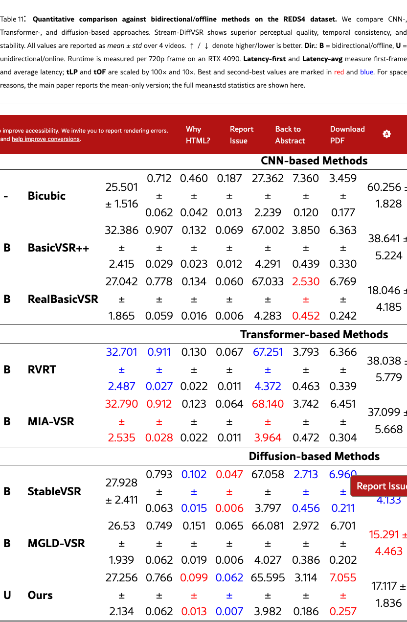
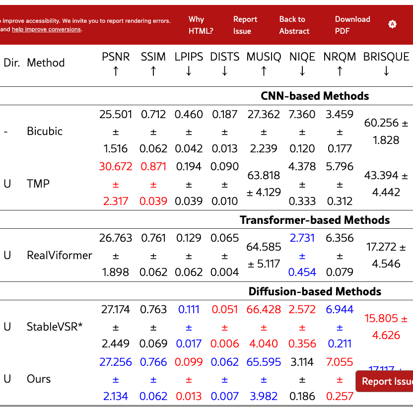
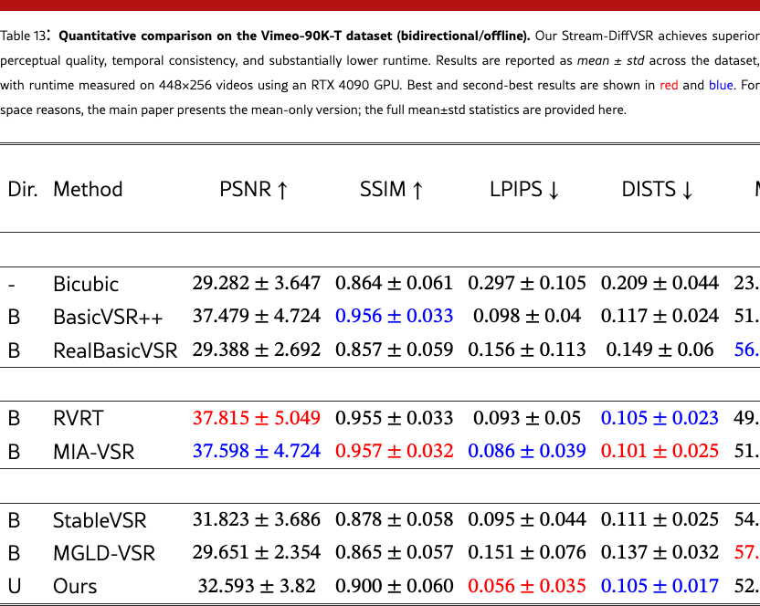
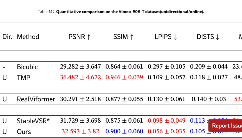
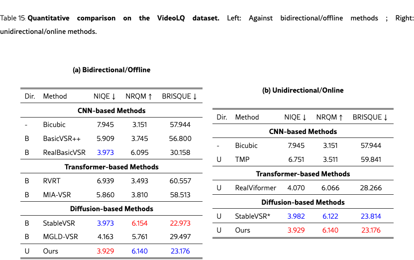
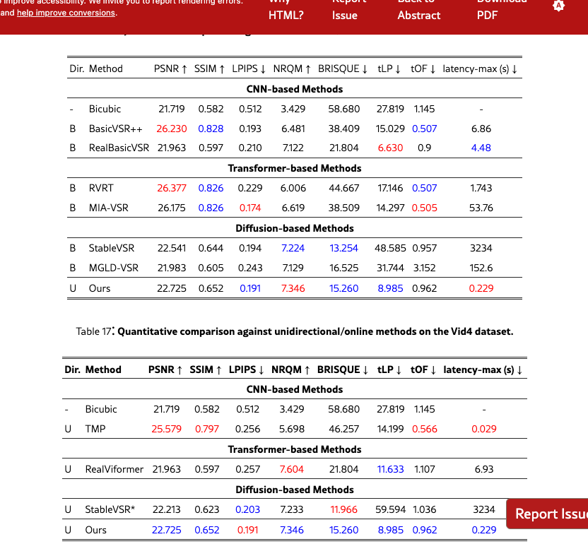
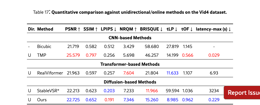
We provide extended quantitative results across multiple datasets and settings. Specifically, we report both bidirectional and unidirectional performance with mean and standard deviation on REDS4 (Tabs. 11 and 12) and Vimeo-90K (Tabs. 13 and 14), while additional bidirectional results are provided on VideoLQ (Tab. 15) and Vid4 (Tabs. 17 and 17). These supplementary results further validate the robustness of our approach under diverse benchmarks and temporal settings.

A4.T15 — Table 15:Quantitative comparison on the VideoLQ dataset. Left: Against bidirectional/offline methods ; Right: unidirectional/online methods.

A4.T17 — Table 16:Quantitative comparison against bidirectional/offline methods on the Vid4 dataset.

A4.T17.16 — Table 17:Quantitative comparison against unidirectional/online methods on the Vid4 dataset.

Appendix E Additional Visual Result

A5.F9 — Figure 9:Qualitative comparison with Upscale-A-Video (UAV). Due to GPU memory limitations (OOM on an RTX 4090), we use UAV results extracted from its official project video for qualitative comparison. Despite this constraint, our Stream-DiffVSR exhibits superior visual fidelity and temporal consistency across frames.

A5.F10 — Figure 10:Additional visual results.

A5.F11 — Figure 11:Additional visual results.

A5.F12 — Figure 12:Additional visual results.

A5.F13 — Figure 13:Temporal consistency comparison. Qualitative comparison of temporal consistency across consecutive frames. Our proposed Stream-DiffVSR effectively mitigates flickering artifacts and maintains stable texture reconstruction, demonstrating superior temporal coherence compared to existing VSR methods.

A5.F14 — Figure 14:Optical flow visualization comparison. Visualization of optical flow consistency across different VSR methods. Our proposed Stream-DiffVSR produces smoother and more temporally coherent flow fields, indicating improved motion consistency and reduced temporal artifacts compared to competing approaches.

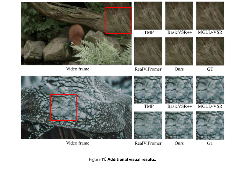
Figs. 10, 11 and 12 presents qualitative results on challenging real-world sequences. Compared with CNN-based (TMP, BasicVSR++) and Transformer-based (RealViFormer) approaches, as well as the diffusion-based MGLD-VSR, our method produces sharper structures and more faithful textures while effectively reducing temporal flickering. These visual comparisons further demonstrate the effectiveness of our design in maintaining perceptual quality and temporal consistency across diverse scenes.

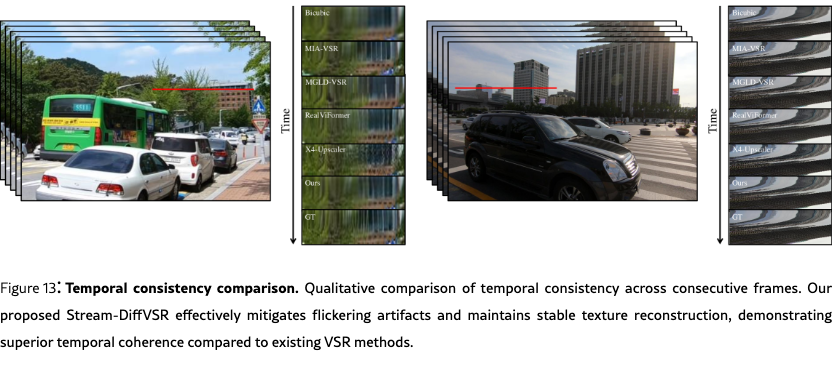
Temporal consistency comparison. As shown in the consecutive-frame comparisons Fig. 13, Stream-DiffVSR alleviates flickering artifacts and preserves stable textures over time, yielding noticeably stronger temporal coherence than prior VSR methods.

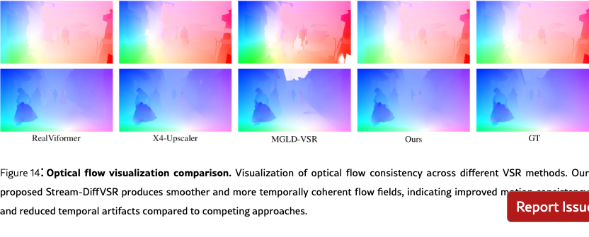
Optical flow visualization comparison. The optical flow consistency visualizations Fig. 14 further highlight our advantages: Stream-DiffVSR generates smoother and more temporally coherent flow fields, reflecting improved motion stability and reduced temporal artifacts.

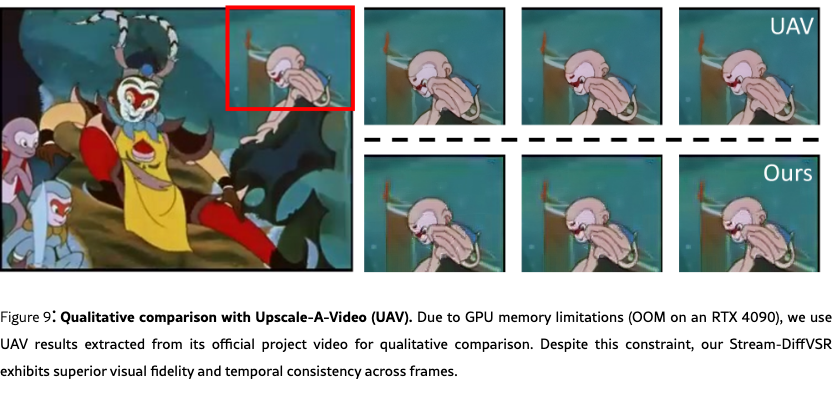
We also provide qualitative comparisons with Upscale-A-Video [104] in Fig. 9. Owing to GPU memory constraints, the official model cannot be executed locally, so we rely on frames extracted from its project video. Despite this limitation, Stream-DiffVSR demonstrates superior fine-detail reconstruction and notably improved temporal stability in UAV scenarios.

Appendix F Failure cases

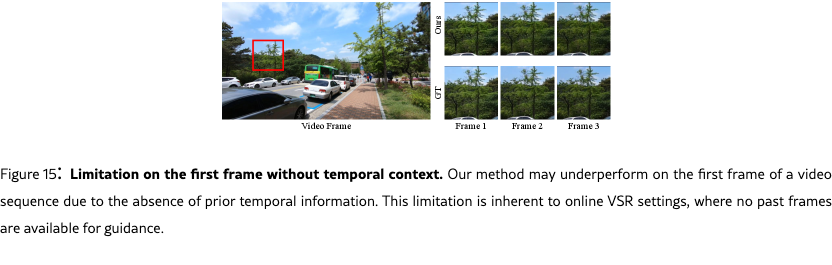
A6.F15 — Figure 15: Limitation on the first frame without temporal context. Our method may underperform on the first frame of a video sequence due to the absence of prior temporal information. This limitation is inherent to online VSR settings, where no past frames are available for guidance.

Fig. 15 illustrates a limitation of our approach on the first frame of a video sequence. Since no past frames are available for temporal guidance, the model may produce blurrier details or less stable structures compared to subsequent frames. This issue is inherent to all online VSR settings, where temporal information cannot be exploited at the sequence start. As shown in later frames, once temporal context becomes available, our method quickly stabilizes and reconstructs high-fidelity details.