]ByteDance Seed \contribution[†]Project Lead \contribution[*]Equal Contribution
Depth Anything 3:
Recovering the Visual Space from Any Views
Abstract
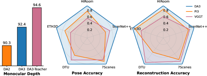
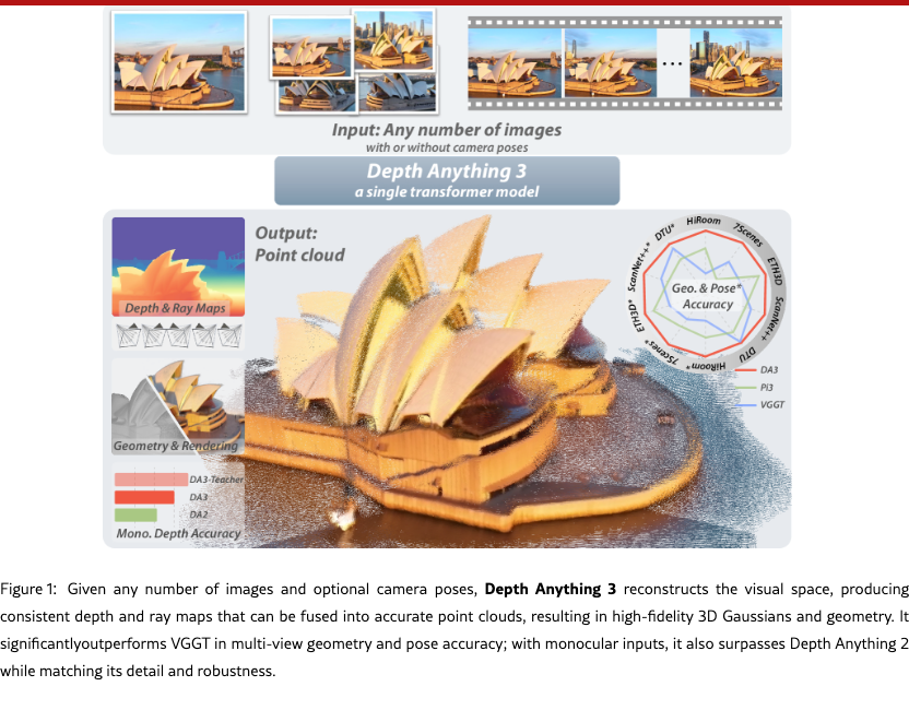
We present Depth Anything 3 (DA3), a model that predicts spatially consistent geometry from an arbitrary number of visual inputs, with or without known camera poses. In pursuit of minimal modeling, DA3 yields two key insights: a single plain transformer (e.g., vanilla DINO encoder) is sufficient as a backbone without architectural specialization, and a singular depth-ray prediction target obviates the need for complex multi-task learning. Through our teacher-student training paradigm, the model achieves a level of detail and generalization on par with Depth Anything 2 (DA2). We establish a new visual geometry benchmark covering camera pose estimation, any-view geometry and visual rendering. On this benchmark, DA3 sets a new state-of-the-art across all tasks, surpassing prior SOTA VGGT by an average of 35.7% in camera pose accuracy and 23.6% in geometric accuracy. Moreover, it outperforms DA2 in monocular depth estimation. All models are trained exclusively on public academic datasets.
Bingyi Kang\checkdata[Project Page]depth-anything-3.github.io
1 Introduction
The ability to perceive and understand 3D spatial information from visual input is a cornerstone of human spatial intelligence [arterberry2000perception] and a critical requirement for applications like robotics and mixed reality. This fundamental capability has inspired a wide array of 3D vision tasks, including Monocular Depth Estimation [eigen2014depth], Structure from Motion [snavely2006photo], Multi-View Stereo [seitz2006comparison] and Simultaneous Localization and Mapping [mur2015orb]. Despite the strong conceptual overlap between these tasks—often differing by only a single factor, such as the number of input views—the prevailing paradigm has been to develop highly specialized models for each one. While recent efforts [wang2024dust3r, wang2025vggt] have explored unified models to address multiple tasks simultaneously, they typically suffer from key limitations: they often rely on complex, bespoke architectures, are trained via joint optimization over tasks from scratch, and consequently cannot effectively leverage large-scale pretrained models.
In this work, we step back from established 3D task definitions and return to a more fundamental goal inspired by human spatial intelligence: recovering 3D structure from arbitrary visual inputs, be it a single image, multiple views of a scene, or a video stream. Forsaking intricate architectural engineering, we pursue a minimal modeling strategy guided by two central questions. First, is there a minimal set of prediction targets, or is joint modeling across numerous 3D tasks necessary? Second, can a single plain transformer suffice for this objective? Our work provides an affirmative answer to both. We present Depth Anything 3, a single transformer model trained exclusively for joint any-view depth and pose estimation via a specially chosen ray representation. We demonstrate that this minimal approach is sufficient to reconstruct the visual space from any number of images, with or without known camera poses.
Depth Anything 3 formulates the above geometric reconstruction target as a dense prediction task. For a given set of input images, the model is trained to output corresponding depth maps and ray maps, each pixel-aligned with its respective input. The architecture to achieve this begins with a standard pretrained vision transformer (e.g., oquab2023dinov2), as its backbone, leveraging its powerful feature extraction capabilities. To handle arbitrary view counts, we introduce a key modification: an input-adaptive cross-view self-attention mechanism. This module dynamically rearranges tokens during the forward pass in selected layers, enabling efficient information exchange across all views. For the final prediction, we propose a new dual DPT head designed to jointly outputs both depth and ray values, by processing the same set of features with distinct fusion parameters. To enhance flexibility, the model can optionally incorporate known camera poses via a simple camera encoder, allowing it to adapt to various practical settings. This overall design results in a clean and scalable architecture that directly inherits the scaling properties of its pretrained backbone.
We train Depth Anything 3 via a teacher-student paradigm to unify diverse training data, which is necessary for a generalist model. Our data sources include varied formats like real-world depth camera captures (e.g., baruch2021arkitscenes), 3D reconstruction (e.g., reizenstein2021common), and synthetic data, where real-world depth may be of poor quality (Fig.˜4). To resolve this, we adopt a pseudo-labeling strategy inspired by prior works [yang2024depth, yang2024depthv2]. Specifically, we train a powerful teacher monocular depth model on synthetic data to generate dense, high-quality pseudo-depth for all real-world data. Crucially, to preserve geometric integrity, we align these dense pseudo-depth maps with the original sparse or noisy depth. This approach proved remarkably effective, significantly enhancing label detail and completeness without sacrificing the geometric accuracy.
To better evaluate our model and track progress in the field, we establish a comprehensive benchmark for assessing geometry and pose accuracy. The benchmark comprises 5 distinct datasets, totaling over 89 scenes, ranging from object-level to indoor and outdoor environments. By directly evaluating pose accuracy across scenes and fusing the predicted pose and depth into a 3D point cloud for accuracy assessment, the benchmark faithfully measures the pose and depth accuracy of visual geometry estimators. Experiments show that our model achieves state-of-the-art performance on 18 out of 20 settings. Moreover, on standard monocular benchmarks, our model outperforms Depth Anything 2 [yang2024depthv2].
To further demonstrate the fundamental capability of Depth Anything 3 in advancing other 3D vision tasks, we introduce a challenging benchmark for feed-forward novel view synthesis (FF-NVS), comprising over 160 scenes. We adhere to the minimal modeling strategy and fine-tune our model with an additional DPT head to predict pixel-aligned 3D Gaussian parameters. Extensive experiments yield two key findings: 1) fine-tuning a geometry foundation model for NVS substantially outperforms highly specialized task-specific models [xu2025depthsplat]; 2) enhanced geometric reconstruction capability directly correlates with improved FF-NVS performance, establishing Depth Anything 3 as the optimal backbone for this task.
2 Related Work
Multi-view visual geometry estimation.
Traditional systems [schoenberger2016sfm, schoenberger2016mvs] decompose reconstruction into feature detection and matching, robust relative pose estimation, incremental or global SfM with bundle adjustment, and dense multi-view stereo for per-view depth and fused point clouds. These methods remain strong on well-textured scenes, but their modularity and brittle correspondences complicate robustness under low texture, specularities, or large viewpoint changes. Early learning methods injected robustness at the component level: learned detectors [detone2018superpoint], descriptors for matching [dusmanu2019d2], and differentiable optimization layers that expose pose/depth updates to gradient flow [he2024detector, guo2025multi, pan2024global]. On the dense side, cost-volume networks [yao2018mvsnet, xu2023iterative] for MVS replaced hand-crafted regularization with 3D CNNs, improving depth accuracy especially at large baselines and thin structures compared with classical PatchMatch. Early end-to-end approaches [teed2018deepv2d, wang2024vggsfm] moved beyond modular SfM/MVS pipelines by directly regressing camera poses and per-image depths from pairs of images. These approaches reduced engineering complexity and demonstrated the feasibility of learned joint depth pose estimation, but they often struggled with scalability, generalization, and handling arbitrary input cardinalities.
A turning point came with DUSt3R [dust3r], which leveraged transformers to directly predict point map between two views and compute both depth and relative pose in a purely feed-forward manner. This work laid the foundation for subsequent transformer-based methods aiming to unify multi-view geometry estimation at scale. Follow-up models extended this paradigm with multi-view inputs [fast3r, cut3r, Mv-dust3r+, must3r], video input [monst3r, cut3r, murai2025mast3r, deng2025vggtlong], robust correspondence modeling [mast3r], camera parameter injection [jang2025pow3r, keetha2025mapanything], large-scale SfM [deng2025sailrecon], SLAM applications [maggio2025vggtslam], and view synthesis with 3D Gaussians [flare, smart2024splatt3r, charatan2024pixelsplat, chen2024mvsplat, jiang2025anysplat, xu2025depthsplat]. Among these, [wang2025vggt] push accuracy to a new level through large-scale training, a multi-stage architecture, and redundancy in design. In contrast, we focus on a minimal modeling strategy built around a single, simple transformer.
Monocular depth estimation.
Early monocular depth estimation methods relied on fully supervised learning on single-domain datasets, which often produced models specialized to either indoor rooms [silberman2012indoor] or outdoor driving scenes [geiger2013vision]. These early deep models achieved good accuracy within their training domain but struggled to generalize to novel environments, highlighting the challenge of cross-domain depth prediction. Modern generalist approaches [yang2024depth, yang2024depthv2, wang2025moge, bochkovskii2024depth, yin2023metric3d, ke2024repurposing] exemplify this trend by leveraging massive multi-dataset training and advanced architectures like vision transformers [ranftl2021vision] or DiT [peebles2023scalable]. Trained on millions of images, they learn broad visual cues and incorporate techniques such as affine-invariant depth normalization. In contrast, our method is primarily designed for a unified visual geometry estimation task, yet it still demonstrates competitive monocular depth performance.
Feed-Forward Novel View Synthesis
Novel view synthesis (NVS) has long been a core problem in computer vision and graphics [levoy1996light, heigl1999plenoptic, buehler2001unstructured], and interest has increased with the rise of neural rendering [sitzmann2019scene, sitzmann2021light, mildenhall2020nerf, kerbl20233d, govindarajan2025radiant]. A particularly promising direction is feed-forward NVS, which produces 3D representations in a single pass through an image-to-3D network, avoiding tedious per-scene optimization. Early methods adopted NeRF as the underlying 3D representation [yu2021pixelnerf, chen2021mvsnerf, lin2022efficient, chen2025explicit, hong2024lrm, xu2024murf], but recent work has largely shifted to 3DGS due to its explicit structure and real-time rendering. Representative approaches improve image-to-3D networks with geometry priors, e.g., epipolar attention [charatan2024pixelsplat], cost volumes [chen2024mvsplat], and depth priors [xu2024murf]. More recently, multi-view geometry foundation models [dust3r, Mv-dust3r+, fast3r, wang2025vggt] have been integrated to improve modeling capacity, particularly in pose-free settings, yet methods built upon such models are often evaluated by relying on a single chosen foundation model [smart2024splatt3r, ye2024no, jiang2025anysplat]. Here, we systematically benchmark the contribution of different geometry foundation models to NVS and propose strategies to better exploit them, enabling feed-forward 3DGS to handle both posed and pose-free inputs, variable numbers of views, and arbitrary resolutions.
3 Depth Anything 3
We tackle the recovery of consistent 3D geometry from diverse visual inputs—single image, multi-view collections, or videos—and optionally incorporate known camera poses when available.
3.1 Formulation
We denote the input as with each . For this is a monocular image, and for it represents a video or multi-view set. Each image has depth , camera extrinsics , and intrinsics . The camera can also be represented as with translation , rotation quaternion , and FOV parameters . A pixel projects to a 3D point by
through which the underlying 3D visual space can be faithfully recovered.
Depth-ray representation.
Predicting a valid rotation matrix is challenging due to the orthogonality constraint. To avoid this, we represent camera pose implicitly with a per-pixel ray map, aligned with the input image and depth map. For each pixel , the camera ray is defined by its origin and direction : . The direction is obtained by backprojecting into the camera frame and rotating it to the world frame: The dense ray map stores these parameters for all pixels. We do not normalize , so its magnitude preserves the projection scale. Thus, a 3D point in world coordinates is simply This formulation enables consistent point cloud generation by combining predicted depth and ray maps through element-wise operations.
Deriving Camera Parameters from the Ray Map.
Given an input image , the corresponding ray map is denoted by . This map comprises per-pixel ray origins, stored in the first three channels (), and ray directions, stored in the last three ().
First, the camera center is estimated by averaging the per-pixel ray origin vectors:
| (1) |
To estimate the rotation and intrinsics , we formulate the problem as finding a homography . We begin by defining a “identity” camera with an identity intrinsics matrix, . For a given pixel , its corresponding ray direction in this canonical camera’s coordinate system is simply . The transformation from this canonical ray to the ray direction in the target camera’s coordinate system is given by . This establishes a direct homography relationship, , between the two sets of rays. We can then solve for this homography by minimizing the geometric error between the transformed canonical rays and a set of pre-computed target rays, . This leads to the following optimization problem:
| (2) |
This is a standard least-squares problem that can be efficiently solved using the Direct Linear Transform (DLT) algorithm [abdel2015direct]. Once the optimal homography is found, we recover the camera parameters. Since the intrinsic matrix is upper-triangular and the rotation matrix is orthonormal, we can uniquely decompose using RQ decomposition to obtain , .
Minimal prediction targets.
Recent works aim to build unified models for diverse 3D tasks, often using multitask learning with different targets—for example, point maps alone [dust3r], or redundant combinations of pose, local/global point maps, and depth [wang2025vggt, cut3r, fast3r]. While point maps are insufficient to ensure consistency, redundant targets can improve pose accuracy but often introduce entanglement that compromises it. In contrast, our experiments (Tab.˜6) show that a depth-ray representation forms a minimal yet sufficient target set for capturing both scene structure and camera motion, outperforming alternatives like point maps or more complex outputs. However, recovering camera pose from the ray map at inference is computationally costly. We address this by adding a lightweight camera head, . This transformer operates on camera tokens to predict the field of view (), rotation as a quaternion (), and translation (). Since it processes only one token per view, the added cost is negligible.
3.2 Architecture
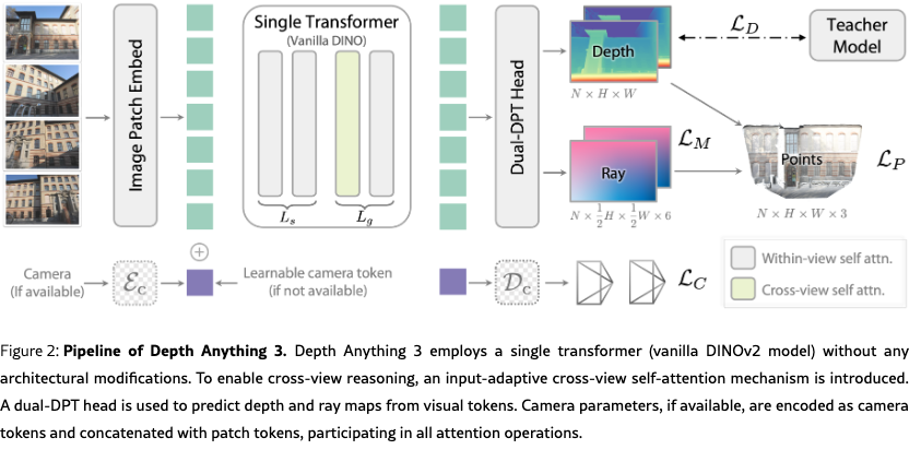
We now detail the architecture of Depth Anything 3, which is illustrated in Fig.˜2. The network is composed of three main components: a single transformer model as the backbone, an optional camera encoder for pose conditioning, and a Dual-DPT head for generating predictions.
Single transformer backbone. We use a Vision Transformer with blocks, pretrained on large-scale monocular image corpora (e.g., DINOv2 [oquab2023dinov2]). Cross-view reasoning is enabled without architectural changes via an input-adaptive self-attention, implemented by rearranging input tokens. We divide the transformer into two groups of sizes and . The first layers apply self-attention within each image, while the subsequent layers alternate between cross-view and within-view attention, operating on all tokens jointly through tensor reordering. In practice, we set with . As shown in our ablation study in Tab.˜7, this configuration provides the optimal trade-off between performance and efficiency compared to other arrangements. This design is input-adaptive: with a single image, the model naturally reduces to monocular depth estimation without extra cost.
Camera condition injection. To seamlessly handle both posed and unposed inputs, we prepend each view with a camera token . If camera parameters are available, the token is obtained via a lightweight MLP : . Otherwise, a shared learnable token is used. Concatenated with patch tokens, these camera tokens participate in all attention operations, providing either explicit geometric context or a consistent learned placeholder.
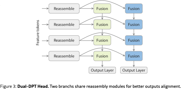
Dual-DPT head. For the final prediction stage, we propose a novel Dual-DPT head that jointly produces dense depth and ray values. As shown in Tab.˜6, this design is both powerful and efficient. Given a set of features from the backbone, the Dual-DPT head first processes them through a shared set of reassembly modules. Subsequently, the processed features are fused using two distinct sets of fusion layers: one for the depth branch and one for the ray branch. Finally, two separate output layers produce the final depth and ray map predictions. This architecture ensures that both branches operate on the same set of processed features, differing only in the final fusion stage. Such a design encourages strong interaction between the two prediction tasks, while avoiding redundant intermediate representations.
3.3 Training
Teacher-student learning paradigm. Our training data comes from diverse sources, including real-world depth captures, 3D reconstructions, and synthetic datasets. Real-world depth is often noisy and incomplete (Fig.˜4), limiting its supervisory value. To mitigate this, we train a monocular relative depth estimation “teacher” model solely on synthetic data to generate high-quality pseudo-labels. These pseudo-depth maps are aligned with the original sparse or noisy ground truth via RANSAC least squares, enhancing label detail and completeness while preserving geometric accuracy. We term this model Depth-Anything-3-Teacher, trained on a large synthetic corpus covering indoor, outdoor, object-centric, and diverse in-the-wild scenes to capture fine geometry. We detail our teacher design in the Sec.˜4.1.
Training objectives.
Following the formulation in Sec.˜3.1, our model maps an input to a set of outputs comprising a depth map , a ray map , and an optional camera pose : . The gray color indicates that is an optional output, included primarily for practical convenience. Prior to loss computation, all ground-truth signals are normalized by a common scale factor. This scale is defined as the mean norm of the valid reprojected point maps , a step that ensures consistent magnitude across different modalities and stabilizes the training process. The overall training objective is defined as a weighted sum of several terms:
where denotes the confidence of depth . All loss terms are based on the norm, with weights set to and . The gradient loss, , penalizes the depth gradients:
| (3) |
where and are the horizontal and vertical finite difference operators. This loss preserves sharp edges while ensuring smoothness in planar regions. In practice, we set and .
3.4 Implementation Details
Traing datasets.
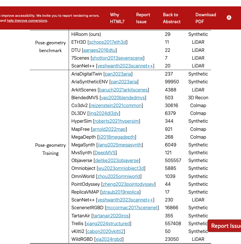
We provide our training datasets in Table 1. Note that for datasets with potential overlap between training and testing (ScanNet++), we ensure a strict separation at the scene level, i.e., scenes in training and testing are mutually exclusive. Note that using Scannet++ for training is fair to other methods, as it is widely used for training in [wang2025vggt, dust3r].
Training details.
We train our model on 128 H100 GPUs for 200k steps, using an 8k-step warm-up and a peak learning rate of . The base resolution is , which is divisible by 2, 3, 4, 6, 9 and 14, making it more compatible with common photo aspect ratios such as 2:3, 3:4, and 9:16. Training image resolutions are randomly sampled from , , , , , , , . For the resolution, the number of views is sampled uniformly from [2, 18]. The batch size is dynamically adjusted to keep the token count per step approximately constant. Supervision transitions from ground-truth depth to teacher-model labels at 120k steps. Pose conditioning is randomly activated during training with probability 0.2.
4 Teacher-Student Learning
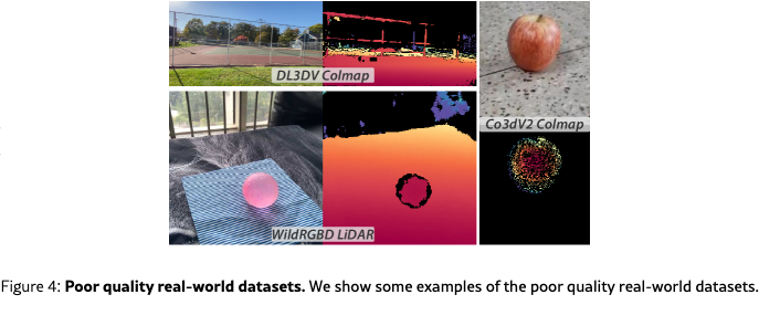
As shown in Fig.˜4, the real-world datasets are of poor quality, thus we train the teacher model exclusively on synthetic data to provide supervision for real-world data. Our teacher model is trained as a monocular relative depth predictor. During inference or supervision, noisy ground-truth depth can be used to provide scale and shift parameters, allowing for the alignment of the predicted relative depth with absolute depth measurements.
4.1 Constructing the Teacher Model
Building upon Depth Anything 2 [yang2024depth], we extend the approach in several key aspects, including both data and representation. We observe that expanding the training corpus yields clear improvements in depth estimation performance, substantiating the benefits of data scaling. Furthermore, while our revised depth representation may not show striking improvements on standard 2D evaluation metrics, it leads to qualitatively better 3D point clouds, exhibiting fewer geometric distortions and more realistic scene structures. It is important to note that our teacher network backbone is directly aligned with the above DA3 framework, consisting solely of a DINOv2 vision transformer with a DPT decoder—no specialized architectural modifications are introduced. We elaborate on the full design and implementation details in the following sections.
Data scaling. We train the teacher model exclusively on synthetic data to achieve finer geometric detail. The synthetic datasets used in DA2 are relatively limited. In DA3, we substantially expand the training corpus to include: Hypersim [roberts2021hypersim], TartanAir [tartanair2020iros], IRS [wang2019irs], vKITTI2 [cabon2020vkitti2], BlendedMVS [yao2020blendedmvs], SPRING [mehl2023spring], MVSSynth [DeepMVS], UnrealStereo4K [zhang2018unrealstereo], GTA-SfM [wang2020flow], TauAgent [gil2021online], KenBurns [niklaus20193d], MatrixCity [li2023matrixcity], EDEN [le2021eden], ReplicaGSO [replica19arxiv], UrbanSyn [GOMEZ2025130038], PointOdyssey [zheng2023pointodyssey], Structured3D [zheng2020structured3d], Objaverse [deitke2023objaverse], Trellis [xiang2024structured], and OmniObject [wu2023omniobject3d]. This collection spans indoor, outdoor, object-centric, and diverse in-the-wild scenes, improving generalization of the teacher model.
Depth representation. Unlike DA2, which predicts scale–shift-invariant disparity, our teacher outputs scale–shift-invariant depth. Depth is preferable for downstream tasks, such as metric depth estimation and multiview geometry, that directly operate in depth space rather than disparity. To address depth’s reduced sensitivity for near-camera regions comparing to disparity, we predict exponential depth instead of linear depth, enhancing discrimination at small distances.
Training objectives. For geometric supervision, in addition to a standard depth-gradient loss, we adopt ROE alignment with the global–local loss introduced in [wang2025moge]. To further refine local geometry, we introduce a distance-weighted surface-normal loss. For each center pixel, we sample four neighboring points and compute unnormalized normals . We then weight these normals by:
| (4) |
which downweights contributions from neighbors farther from the center, yielding a mean normal closer to the true local surface normal:
| (5) |
The final normal loss is
| (6) |
where denotes the angular error between normals. Ground truth is undefined in sky regions and in background areas of object-only datasets. To prevent these regions from degrading the depth prediction and to facilitate downstream use, we jointly predict a sky mask and an object mask aligned with the depth output, supervised with MSE loss. The overall training objective is
| (7) |
where . Here, , , , and denote the gradient loss, global–local loss, sky-mask loss, and object-mask loss, respectively.
4.2 Teaching Depth Anything 3
Real-world datasets are crucial for generalizing camera pose estimation, yet they rarely provide clean depths; supervision is often noisy or sparse (Fig.˜4). Depth Anything 3 Teacher provides high-quality relative depth, which we align to noisy metric measurements (e.g., COLMAP or active sensors) via a robust ransac scale–shift procedure. Let denote the teacher’s relative depth and the available sparse depth with validity mask over domain . We estimate scale and shift by RANSAC least squares, using an inlier threshold equal to the mean absolute deviation from the residual median:
| (8) |
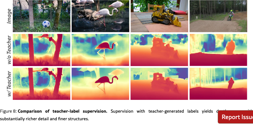
The aligned provides scale-consistent and pose–depth coherent supervision for Depth Anything 3, complementing our joint depth–ray objectives and improving real-world generalization, as evidenced in Fig.˜8.
4.3 Teaching Monocular Model
We additionally train a monocular depth model under a teacher–student paradigm. We follow the DA2 framework, training the monocular student on unlabeled images with teacher-generated pseudo-labels. The key difference from DA2 lies in the prediction target: our student predicts depth maps, whereas DA2 predicts disparity. We further supervise the student with the same loss used for the teacher, applied to the pseudo-depth labels. The monocular model also predicts relative depth. Trained solely on unlabeled data with teacher supervision, it achieves state-of-the-art performance on standard monocular depth benchmarks as shown in Tab.˜10.
4.4 Teaching Metric Model
Next, we demonstrate that our teacher model can be used for training a metric depth estimation model with sharp boundaries. Following Metric3Dv2 [hu2024metric3dv2], we apply canonical camera space transformation to address depth ambiguity caused by varying focal lengths. Specifically, we rescale the ground-truth depth using ratio , where and denote the canonical focal length and camera focal length, respectively. To ensure sharp details, we employ Teacher model’s prediction as training labels. We align the scale and shift of the teacher model’s predicted depths with the ground-truth metric depth labels for supervision.
Training dataset.
We trained our metric depth model on 14 datasets, including Taskonomy [zamir2018taskonomy], DIML (Outdoor) [cho2021diml], DDAD [ddad], Argoverse [wilson2023argoverse], Lyft [], PandaSet [xiao2021pandaset], Waymo [Sun_2020_CVPR], ScanNet++ [yeshwanth2023scannet++], ARKitScenes [baruch2021arkitscenes], Map-free [arnold2022map], DSEC [Gehrig21ral], Driving Stereo [yang2019drivingstereo] and Cityscapes [cordts2016cityscapes] datasets. For stereo datasets, we leverage the prediction of FoundationStereo [wen2025foundationstereo] as training labels.
Implementation Details.
The training largely follows that of the monocular teacher model. All images are trained at a base resolution of 504 with varying aspect ratios (1:1, 1:2, 16:9, 9:16, 3:4, 1:1.5, 1.5:1, 1:1.8). We employ AdamW optimizer and set the learning rate for encoder and decoder to 5e-6 and 5e-5, respectively. We apply random rotation augmentation where training images are rotated at 90 or 270 degree with 5% probability. We set canonical focal length to 300. We use the aligned prediction from teacher model as supervision. With a probability of 20%, we use the original ground-truth labels for training. We train with batch size of 64 for 160K iterations. The training objective is a weighted sum of depth loss , and sky-mask loss .
5 Application: Feed-Forward 3D Gaussian Splattings
5.1 Pose-Conditioned Feed-Forward 3DGS
Inspired by human spatial intelligence, we believe that consistent depth estimation can greatly enhance downstream 3D vision tasks. We choose feed-forward novel view synthesis (FF-NVS) as the demonstration task, given its growing attention driven by advances in neural 3D representations (i.e., we choose 3DGS) and its relevance to numerous applications. Adhere to the minimal modeling strategy, we perform FF-NVS by fine-tuning with an added DPT head (GS-DPT) to infer pixel-aligned 3D Gaussians [charatan2024pixelsplat, chen2024mvsplat].
GS-DPT head. Given visual tokens for each view extracted via our single transformer backbone (Sec.˜3.2), GS-DPT predicts the camera-space 3D Gaussian parameters , where , , , denote the opacity, rotation quaternion, scale, and RGB color of the -th 3D Gaussian, respectively. Among them, is predicted by the confidence head, while others are predicted by the main GS-DPT head. The estimated depth is unprojected to world coordinates to obtain the global positions of the 3D Gaussians. These primitives are then rasterized to synthesize novel views from given camera poses.
Training objectives. The NVS model is fine-tuned with two training objectives, namely photometric loss (i.e., and ) on rendered novel views and scale-shift-invariant depth loss on the estimated depth of observed views, following the teacher–student learning paradigm (Sec.˜3.3).
5.2 Pose-Adaptive Feed-Forward 3DGS
Unlike the above pose-conditioned version intended to benchmark DA3 as a strong feed-forward 3DGS backbone, we also present an alternative better suited to in-the-wild evaluation. This version is designed to integrate seamlessly with DA3 using identical pretrained weights, enabling novel view synthesis with or without camera poses, and across varying resolutions and input view counts.
Pose-adaptive formulation. Rather than assuming that all input images are uncalibrated [smart2024splatt3r, ye2024no, flare, jiang2025anysplat], we adopt a pose-adaptive design that accepts both posed and unposed inputs, yielding a flexible framework that works with or without poses. Two design choices are required to achieve this: 1) all 3DGS parameters are predicted in local camera space. 2) the backbone must handle posed and unposed images seamlessly. Our DA3 backbone satisfies both requirements (Sec.˜3.2). In particular, when poses are available, we scale (via [umeyama2002least]) and unproject the predicted depth and camera-space 3DGS to world space to align with them. When poses are not available, we directly use the predicted poses for the unprojection to world space.
To reduce the trade-off between accurate surface geometry and rendering quality [guedon2024sugar], we predict an additional depth offset in the GS-DPT head. For more in-the-wild robustness, we replace per 3D Gaussian color with spherical harmonic coefficients to reduce conflicts with geometry via modeling view-dependent surface.
Enhanced training strategies. To avoid unstable training, we initialize the DA3 backbone from pretrained weights and freeze it when training, tuning only the GS-DPT head. To improve in-the-wild performance, we train with varying image resolutions and varying numbers of context views. Specifically, higher-resolution inputs are paired with fewer context views and lower-resolution inputs with more views, which stabilizes training while supporting diverse evaluation scenarios.
5.3 Implementation Details
Training datasets.
For training the NVS model, we leverage the large-scale DL3DV dataset [ling2024dl3dv], which provides diverse real-world scenes with camera poses estimated by COLMAP. We use 10,015 scenes from DL3DV for training the feed-forward 3DGS model. To ensure fair evaluation, we strictly maintain exclusivity between training and testing splits: the 140 DL3DV scenes used for benchmarking are completely disjoint from the training set, preventing any data leakage.
6 Visual Geometry Benchmark
We further introduce a visual geometry benchmark to assess geometry prediction models. It directly evaluates pose accuracy, depth via reconstruction accuracy and visual rendering quality.
6.1 Benchmark Pipeline
Pose estimation.
For each scene, we select all available images; if the total number exceeds the limit, we randomly sample 100 images using a fixed random seed. The selected images are then processed through a feed-forward model to generate consistent pose and depth estimations, after which the pose accuracy is computed.
Geometry estimation.
For the same image set, we perform reconstruction using the predicted poses together with the predicted depths. To align the reconstructed point cloud with the ground-truth, we employ evo [umeyama2002least] to align the predicted poses to the ground-truth poses, obtaining a transformation that maps the reconstruction into the ground-truth coordinate system. To improve robustness, we adopt a RANSAC-based alignment procedure. Specifically, we repeatedly apply evo on randomly sampled pose subsets and evaluate each candidate transformation by counting the number of inlier poses, where inliers are defined as those with translation errors below the median of the overall pose deviations. The transformation with the largest inlier set is then chosen and applied to fuse the aligned predicted point cloud with the predicted depth maps by TSDF fusion. Finally, reconstruction quality is assessed by comparing the aligned reconstruction with the ground-truth point cloud using the metrics described in Sec. 6.2.
Visual rendering.
For each testing scene, the number of images typically ranges from 300 to 400 across all benchmark datasets. We sample one out of every 8 images as target novel views for evaluation. From the remaining viewpoints, we use COLMAP camera poses provided by each dataset and apply farthest point sampling, considering both camera translation and rotation distances, to select 12 images as input context views. For DL3DV, we use the official Benchmark set for testing. For Tanks and Temples, all Training Data scenes are included except Courthouse. For MegaDepth, we select scenes numbered from 5000 to 5018, as these are most suitable for NVS.
6.2 Metrics
Pose metrics.
For assessing pose estimation, we follow the evaluation protocol introduced in [wang2025vggt, wang2023posediffusion] and report results using the AUC. This metric is derived from two components: Relative Rotation Accuracy (RRA) and Relative Translation Accuracy (RTA). RRA and RTA quantify the angular deviation in rotation and translation, respectively, between two images. Each error is compared against a set of thresholds to obtain accuracy values. AUC is then computed as the integral of the accuracy–threshold curve, where the curve is determined by the smaller of RRA and RTA at each threshold. To illustrate performance under different tolerance levels, we primarily report results at thresholds of 3 and 30.
Reconstrution metrics.
Let denote the ground-truth point set and the reconstructed point set under evaluation. We measure accuracy using and completeness using following [aanaes2016dtu]. The Chamfer Distance (CD) is then defined as the average of these two terms. Based on these distances, we define the precision and recall of the reconstruction with respect to a distance threshold . Precision is given by , and recall by , where denotes the Iverson bracket [knapitsch2017tnt]. To jointly capture both measures, we report the F1-score, computed as .
6.3 Datasets
Our benchmark is built on five datasets: HiRoom [SVLightVerse2025], ETH3D [schops2017eth3d], DTU [aanaes2016dtu], 7Scenes [shotton2013sevenscene], and ScanNet++ [yeshwanth2023scannet++]. Together, they cover diverse scenarios ranging from object-centric captures to complex indoor and outdoor environments, and are widely adopted in prior research. Below, we present more details about the dataset preparation process.
HiRoom is a Blender-rendered synthetic dataset comprising 30 indoor living scenes created by professional artists. We use a threshold of 0.05m for the F1 reconstruction metric calculation. For TSDF fusion, we set the parameters voxel size to 0.007m.
ETH3D provides high-resolution indoor and outdoor images with ground-truth depth from laser sensors. We aggregate the ground-truth depth maps with TSDF fusion for GT 3D shapes. We select 11 scenes: courtyard, electro, kicker, pipes, relief, delivery area, facade, office, playground, relief 2, terrains, for the benchmark. All frames are used in the evaluation. We use a threshold of 0.25 for the F1 reconstruction metric calculation. For TSDF fusion, we set the parameters voxel size to 0.039m.
DTU is an indoor dataset consisting of 124 different objects, each scene is recorded from 49 views. It provides ground-truth point clouds collected under well-controlled conditions. We evaluate models on the 22 evaluation scans of the DTU dataset following [yao2018mvsnet]. We adopt the RMBG 2.0 [BiRefNet] to remove meaningless background pixels and use the default depth fusion strategy proposed in [zhang2023geomvsnet]. All frames are used in the evaluation.
7Scenes is a challenging real-world dataset, consisting of low-resolution images with severe motion blurs for in-door scenes. We follow the implementation in [zhu2024nicerslam] to fuse RGBD images with TSDF fusion and prepare ground-truth 3D shapes. We downsample the number of frames for each scene by 11 to faciliate evaluation. We use a threshold of 0.05m for the F1 reconstruction metric calculation. For TSDF fusion, we set the parameters voxel size to 0.007m.
ScanNet++ is an extensive indoor dataset providing high-resolution images, depth maps from iPhone LiDAR, and high-resolution depth maps sampled from reconstructions of laser scans. We select 20 scenes for the benchmark. As depth maps from iPhone LiDAR lack of invalid ground-truth indicators, we use depth maps sampled from reconstructions of laser scans as ground-truth depth by default. We aggregate the ground-truth depth maps with TSDF fusion for GT 3D shapes. We downsample the number of frames for each scene by 5 to faciliate evaluation. We use a threshold of 0.05m for the F1 reconstruction metric calculation. For TSDF fusion, we set the parameters voxel size to 0.02m.
Visual rendering quality.
We evaluate visual rendering quality on diverse large-scale scenes. We introduce a new NVS benchmark built from three datasets, including DL3DV [ling2024dl3dv] with 140 scenes, Tanks and Temples [knapitsch2017tanks] with 6, and MegaDepth [li2018megadepth] with 19, each spanning around 300 sampled frames. Ground truth camera poses, estimated with COLMAP, are used directly to ensure accurate and fair comparison across diverse models. We report PSNR, SSIM, and LPIPS metrics on rendered novel views using given camera poses.
7 Experiments
7.1 Comparison with State of the Art
Baselines.
VGGT [wang2025vggt] is an end-to-end transformer that jointly predicts camera parameters, depth, and 3D points from one or many views. Pi3 [wang2025pi3] further adopts a permutation-equivariant design to recover affine-invariant cameras and scale-invariant point maps from unordered images. MapAnything [keetha2025mapanything] provides a feed-forward framework that can also take camera pose as input for dense geometric prediction. Fast3R [yang2025fast3r] extends point-map regression to hundreds or even thousands of images in a single forward pass. Finally, DUSt3R [wang2024dust3r] tackles uncalibrated image pairs by regressing point maps and aligning them globally. Our method is similar to VGGT [wang2025vggt], but adopts a new architecture and a different camera representation, and it is orthogonal to Pi3 [wang2025pi3].
Pose estimation.
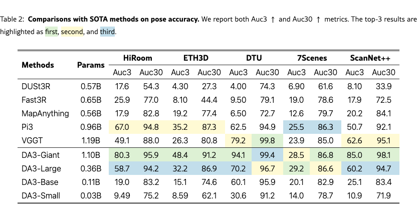
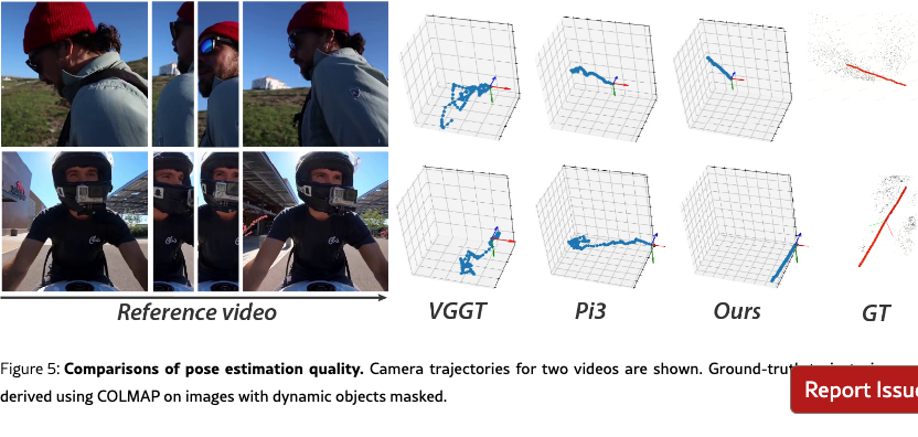
As shown in Tab.˜2 and Fig.˜5, comparing against five baselines [dust3r, wang2025vggt, fast3r, wang2025pi3, keetha2025mapanything], our DA3-Giant model attains the best performance on nearly all metrics, with the only exception being Auc30 on the DTU dataset. Notably, on Auc3 our model delivers at least an relative improvement over all competing methods, and on ScanNet++ it achieves a relative gain over the second-best model.
Geometry estimation.
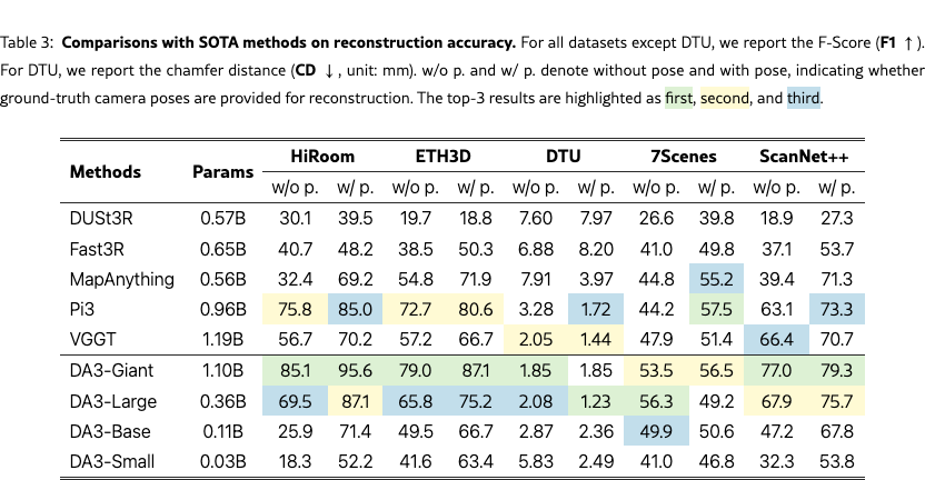
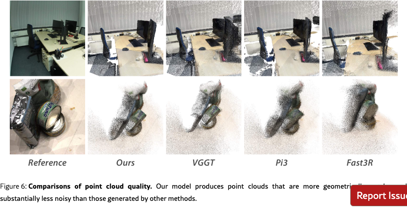
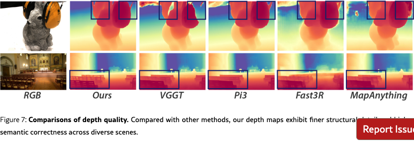
As shown in Tab.˜3, our DA3-Gaint establishes a new SOTA in nearly all scenarios, outperforming all competitors in all five pose-free settings. On average, DA3-Gaint achieves a relative improvement of 25.1% over VGGT and 21.5% over Pi3. Fig.˜7 and Fig.˜6 visualize our predicted depth and recovered point clouds. The results are not only clean, accurate, and complete, but also preserve fine-grained geometric details, clearly demonstrating a superiority over other methods. Even more notably, our much smaller DA3-Large (0.30B parameters) demonstrates remarkable efficiency. Despite being 3 smaller, it surpasses the prior SOTA VGGT (1.19B parameters) in five out of the ten settings, with particularly strong performance on the ETH3D.
When camera poses are available, both our method and MapAnything can exploit them for improved results, and other methods also benefit from ground-truth pose fusion. Our model shows clear gains on most datasets except 7Scenes, where the limited video setting already saturates performance and reduces the benefit of pose conditioning. Notably, with pose conditioning, performance gains from scaling model size are smaller than in pose-free models, indicating that pose estimation scales more strongly than depth estimation and requires larger models to fully realize improvements.
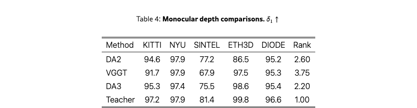
Monocular depth accuracy also reflects geometry quality. As shown in Tab.˜4, on the standard monocular depth benchmarks reported in [yang2024depthv2], our model outperforms VGGT and Depth Anything 2. For reference, we also include the results of our teacher model.
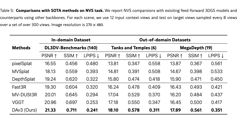
Visual rendering.
To fairly evaluate feed-forward novel view synthesis (FF-NVS), we compare against three recent 3DGS models—pixelSplat [charatan2024pixelsplat], MVSplat [chen2024mvsplat], and DepthSplat [xu2025depthsplat]—and further test alternative frameworks by replacing our geometry backbone with Fast3R [yang2025fast3r], MV-DUSt3R [Mv-dust3r+], and VGGT [wang2025vggt]. All models are trained on DL3DV-10K training set under a unified protocol and evaluated on our benchmark (Sec.˜6.3).
As reported in Tab.˜5, all models perform substantially better on DL3DV than on the other datasets, suggesting that 3DGS-based NVS is sensitive to trajectory and pose distributions standardized by DL3DV, rather than scene content. Comparing the two groups, geometry-model-based frameworks consistently outperform specialized feed-forward models, demonstrating that a simple backbone plus DPT head can surpass complex task-specific designs. The advantage stems from large-scale pretraining, which enables better generalization and scalability than approaches relying on epipolar transformers, cost volumes, or cascaded modules. Within this group, NVS performance correlates with geometry estimation capability, making DA3 the strongest backbone. Looking forward, we expect FF-NVS can be effectively addressed with simple architectures leveraging pretrained geometry backbones, and that the strong spatial understanding of DA3 will benefit other 3D vision tasks.
7.2 Analysis for Depth Anything 3
Training our DA3-Giant model requires 128H100 GPUs for approximately 10 days. To reduce carbon footprint and computational cost, all ablation experiments reported in this section are conducted using the ViT-L backbone with a maximum of 10 views, requiring approximately 4 days on 32H100 GPUs.
7.2.1 Sufficiency of the Depth-Ray Representation
To validate our depth-ray representation, we compare different prediction combinations summarized in Tab.˜6. All models use a ViT-L backbone, identical training settings (view size: 10, batch size: 128, steps: 120k). We evaluate four heads: 1) 0pt for dense depth maps; 2) pcd for direct 3D point clouds; 3) cam for 9-DoF camera pose ; and 4) our proposed ray, predicting per-pixel ray maps (Sec.˜3.1). The ray head uses a Dual-DPT architecture, while pcd uses a separate DPT head. For models without pcd, point clouds are obtained by combining 0ptwith camera parameters from ray or cam. As shown in Table 6, the minimal 0pt+ ray configuration consistently outperforms 0pt+ pcd + cam and 0pt+ cam across all datasets and metrics, achieving nearly 100% relative gain in Auc3 over 0pt+ cam. Adding an auxiliary cam head (0pt+ ray + cam) yields no further benefit, confirming the sufficiency of the depth-ray representation. We adopt 0pt+ ray + cam as our final representation, as the camera head incurs negligible computational overhead, amounting to approximately 0.1% of the computation cost of the main backbone.

7.2.2 Sufficiency of a Single Plain Transformer
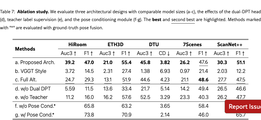
We compare a standard ViT-L backbone with a VGGT-style architecture that stacks two distinct transformers, tripling the block count. For fair capacity comparison, the VGGT-style model uses smaller ViT-B backbones, yielding a similar parameter size to our ViT-L. Our backbone supports two attention strategies: Full Alt., which alternates cross-view/within-view attention in all layers (), and our default partial alternation. As shown in Table 7, the VGGT-style model drops to 79.8% of our baseline performance, confirming the superiority of a single-transformer design at similar scale. We attribute this gap to full pretraining of our backbone versus two-thirds untrained blocks in VGGT. Moreover, the Full Alt. variant degrades across nearly all metrics—except F1 on 7Scenes—indicating that partial alternation is the more effective and robust strategy.
7.2.3 Ablation and Analysis
Dual-DPT Head.
We assess the effectiveness of the dual-DPT head via an ablation in which two separate DPT heads predict depth and ray maps independently. Results are reported in Tab.˜7, item (d). Compared with the model equipped with the dual-DPT head, the variant without it shows consistent drops across metrics, confirming the effectiveness of our dual-DPT design.
Teacher model supervision.
We ablate the use of teacher model labels as supervision, with quantitative results reported in Tab.˜7, item (e). Training without teacher labels yields a slight improvement on DTU but leads to performance drops on 7Scenes and ScanNet++. Notably, the degradation is pronounced on HiRoom. We attribute this to HiRoom’s synthetic nature and its ground truth containing abundant fine structures; supervision from the teacher helps the student capture such details more accurately. Qualitative comparisons in Fig.˜8 corroborate this trend: models trained with teacher-label supervision produce depth maps with substantially richer detail and finer structures.
Pose conditioning.
To assess the pose-conditioning module, we ablate it on the ViT-L backbone and report results in Tab.˜7, items (f) and (g). Unlike other entries in the table, these two are evaluated with ground-truth pose fusion (marked with “*”), whereas the rest use predicted pose fusion. Across metrics, configurations with pose conditioning consistently outperform those without, confirming the effectiveness of the pose-conditioning module.
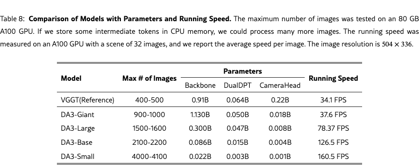
Running time.
We present analysis on Parameters, max number of images and running speed in Tab.˜8
More visualizations.
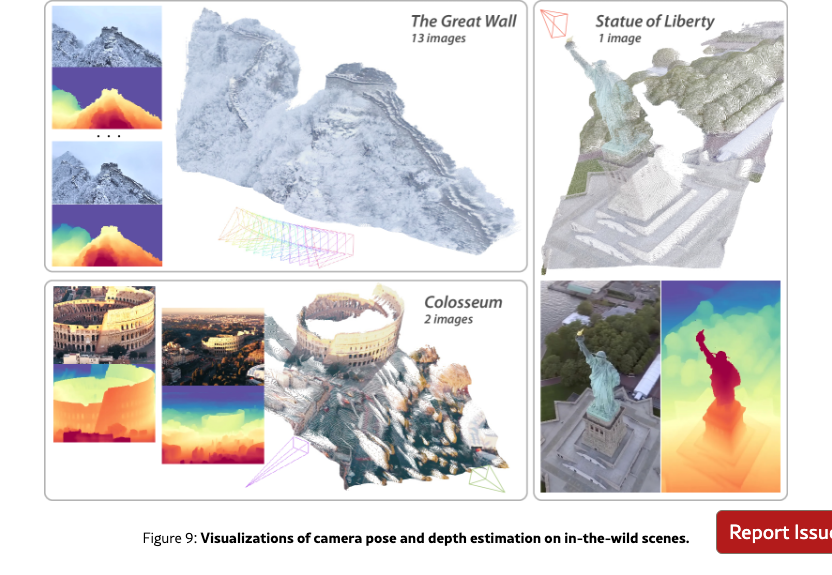
We provide additional visualizations of camera pose and depth estimation on in-the-wild scenes in Fig.˜9, demonstrating the robustness and quality of our model across diverse real-world scenarios.
7.3 Analysis for Depth-Anything-3-Monocular
7.3.1 Teacher Model
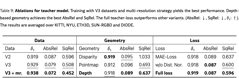
The teacher model’s metrics are reported in Tab.˜4. Our new teacher consistently outperforms DA2 across all datasets, with the sole exception of NYU, where performance is on par with DA2. For the teacher ablation, we employ a ViT-L backbone and a batch size of 64. Evaluation follows the DA2 benchmark protocol, and we additionally report Squared Relative Error (SqRel), defined as the mean squared error between predictions and ground truth normalized by the ground truth. As shown in Tab.˜9, across geometries, depth emerges as the most effective target compared with disparity and point maps. For training objectives, the full teacher loss proposed in this work outperforms both the DA2 loss and a variant without proposed normal-loss term. Finally, data scaling contribute notably to performance: upgrading datasets from V2 to V3 and adopting a multi-resolution training strategy yield consistent improvements in the teacher’s final metrics.
7.3.2 Student Model
As shown in Tab.˜10, our monocular student model with a ViT-L backbone outperforms the DA2 student across all evaluation datasets. Notably, on the ETH3D [schops2017eth3d] benchmark the new monocular student achieves an improvement of over compared with DA2. The improved performance is attributed to the enhanced teacher model with better geometry supervision and the scaled training data (V3). On challenging datasets like SINTEL, our student also demonstrates substantial gains (+5.1%), validating the effectiveness of our teacher-student distillation framework.

7.4 Analysis for Depth-Anything-3-Metric
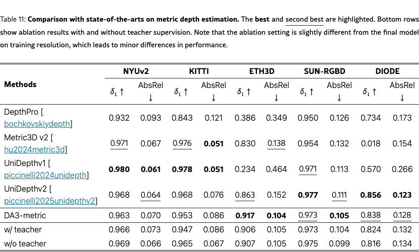
We compare with state-of-the-art metric depth estimation methods, including DepthPro [bochkovskiydepth], Metric3D v2 [hu2024metric3dv2], UniDepthv1 [piccinelli2024unidepth] and UniDepthv2 [piccinelli2025unidepthv2], on 5 benchmarks: NYUv2 [silberman2012nyu], KITTI [geiger2013kitti], ETH3D [schops2017eth3d], SUN-RGBD [song2015sunrgbd] and DIODE (indoor) [vasiljevic2019diode].
As shown in Tab.˜11, DA3-metric achieves state-of-the-art performance on ETH3D ( = 0.917, AbsRel = 0.104), substantially outperforming the second-best method UniDepthv2 ( = 0.863) by a large margin. DA3-metric also achieves best performance on SUN-RGBD for AbsRel (0.105) and second-best on DIODE ( = 0.838, AbsRel = 0.128). While UniDepthv1 and UniDepthv2 achieve the best results on NYUv2 and KITTI, DA3-metric demonstrates strong generalization and competitive performance across all benchmarks, particularly excelling on diverse outdoor scenes like ETH3D.
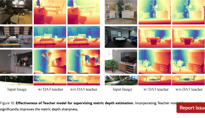
We ablate the Teacher supervision in Tab.˜11. The results show interesting trade-offs: removing Teacher supervision slightly improves metrics on NYUv2 and KITTI, while maintaining comparable performance on other datasets. As shown in Fig. 10, Teacher supervision significantly improves sharpness and fine detail quality, demonstrating that Teacher provides complementary knowledge beyond standard metrics.

7.5 Analysis for Feed-forward 3DGS
We retrain all compared feed-forward 3DGS models, ensuring that the training configuration matches the testing setup by using 12 input context views selected through farthest point sampling. We apply engineering optimizations such as flash attention and fully shared data parallelism to enable all models to process 12 input views efficiently. Depth training loss are incorporated for all baselines to ensure stable training and convergence. All models are trained on 8 A100 GPUs for 200K steps with a batch size of 1, except for pixelSplat, which is trained for 100K steps due to rather slow epipolar attention. All results are reported at .
Visual quality analysis.
We present visual comparisons with other models in Fig.˜11 under novel view synthesis settings. As illustrated, simply augmenting our DA3 model with a 3D Gaussian DPT head yields significantly improved rendering quality over existing state-of-the-art approaches. Our model demonstrates particular strength in challenging regions, such as thin structures (e.g., columns in the first and third scenes) and large-scale outdoor environments with wide-baseline input views (last two scenes), as shown in Fig.˜11. These results underscore the importance of a robust geometry backbone for high-quality visual rendering, consistent with our quantitative findings in Tab.˜5. We anticipate that the strong geometric understanding of DA3 will also benefit other 3D vision tasks.
8 Conclusion and Discussion
Depth Anything 3 shows that a plain transformer, trained on depth-and-ray targets with teacher–student supervision, can unify any-view geometry without ornate architectures. Scale-aware depth, per-pixel rays, and adaptive cross-view attention let the model inherit strong pretrained features while remaining lightweight and easy to extend. On the proposed visual geometry benchmark the approach sets new pose and reconstruction records, with both giant and compact variants surpassing prior models, while the same backbone powers efficient feed-forward novel view synthesis model.
We view Depth Anything 3 as a step toward versatile 3D foundation models. Future work can extend its reasoning to dynamic scenes, integrate language and interaction cues, and explore larger-scale pretraining to close the loop between geometry understanding and actionable world models. We hope the model and dataset releases, benchmark, and simple modeling principles offered here catalyze broader research on general-purpose 3D perception.
Acknowledgement
We thank Xiaowei Zhou, Sida Peng and Hengkai Guo for their valuable discussions during the development of this project. We are also grateful to Yang Zhao for his engineering support. The input images in the teaser demo were extracted from a publicly available YouTube video [mtsdrones2024], credited to the original creator.
While synthetic datasets provide large-scale training data with ground-truth depth annotations, many contain quality issues such as invalid backgrounds, spatial misalignments, clipping artifacts, and erroneous depth values that can degrade model training. We therefore apply careful preprocessing to filter problematic samples and clip unrealistic depth ranges, ensuring high-quality supervision for our teacher model.
Appendix A Data Processing
We preprocess the following raw training datasets as follows to train the teacher model.
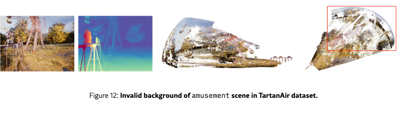
TartanAir.
We remove the amusement scene from training due to its invalid background (skybox) (Fig. 12). We clip the maximum depth values of carwelding, hospital, ocean, office and office2 scenes at 80, 30, 1000, 30 and 30, respectively.
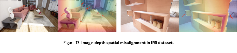
IRS.
We noticed that some of the scenes in IRS exhibit spatial misalignment between the image and depth maps (Fig. 13). To filter those samples with image-depth misalignment, we first run Canny edge detectors on both the image (converted to grayscale) and depth map to extract the boundaries. Next, we dilate the boundaries by 1 pixel and compute the percentage of intersection between image and depth boundaries. Then, we further dilate the boundaries by 3 pixels and compute the intersection between image and depth boundaries. Finally, we compute the ratio between the two intersections and remove samples whose ratio falls below a certain threshold.
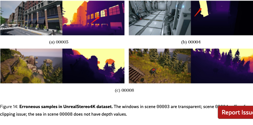
UnrealStereo4K.
We remove the scene 00003 which consists of large erroneous regions. We also remove the scene 00004 which suffers from clipping issue. For scene 00008, we remove samples where the sea does not have depth values (images 9-13, 23-29, 80-82, 86-88, 96, 103-111, 126-136, 144-145, 148-154, 173-176, 178-179, 186-187, 191-192, 198-199) (Fig. 14).
GTA-SfM.
We clip the maximum depth value at 1000.
Kenburns.
We clip the depth value at 50,000 following GitHub issue 111https://github.com/sniklaus/3d-ken-burns/issues/40.
PointOdyssey.
We remove the two scenes animal2_s and dancingroom3_3rd where the ground depth is incorrect 222https://github.com/y-zheng18/point_odyssey/issues/6.
TRELLIS.
We remove all samples with suffix stl, abc, STL, PLY, ply as we noticed that these samples do not contain texture.
OmniObject3D.
We clip the maximum depth value at 10.